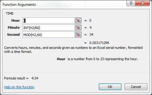
Converting seconds into a minutes:seconds format is rather simple once you know the component parts of the formula. We’ll use three functions. (click to review prior post)
TIME(hour,minute,second)
INT(number)
MOD(number,divisor)
For the TIME Function, the three arguments are:
hour = 0
minute = INT(number)
second = MOD(number, divisor)
Which leaves us with:
TIME(0, INT(number), MOD(number,divisor))
Using 274 seconds as an example, for the INT argument: number = 274/60. The MOD arguments: number = 274, and divisor = 60. Therefore:
=TIME(0,INT(274/60,MOD(274,60))
You can see this applied below, with H2 used as a cell reference for 274, and 60 as the conversion constant.
The TIME Function Argument Dialog Box shows that the function returns 0.003171296, which is the time serial number, and the formula result is 4:34.
When faced with a column of data that shows Time in seconds, the TIME function is useful when combined with the INT and MOD functions. The INT function extracts the number of minutes when the Time(Sec) is divided by 60 seconds per minute, and the MOD function gives the remaining seconds, given the number of seconds and the divisor 60.
In this particular spreadsheet the Hour argument will always be zero because the data happens to be song duration from an iTunes playlist. In a future post I will show and explain the arguments for when Time in seconds is greater than one hour.
The next post will deal with accumulating the TIME data.


So I have a formula in a spreadsheet (see below) that is supposed to return the *days*, hours and minutes of annual leave time I have “banked”.
=TEXT(INT(J63*2.4)+MOD(J63,5/12),”d:hh:mm”)
J63, which is formatted [h]:mm, contains a “number” which represents the total hours and minutes (not days) of leave time I have. Since I work 10-hour days, the formula I have above is supposed to calculate how many *days* (keeping in mind that my day is 10 hours long), hours and seconds J63 represents.
However, something’s not working right. if J63 is 40:00, the formula returns 4:10:00 when it should simply return 4:00:00. 80:00 returns 8:10:00 when it should only be 8. If J63 is a “round” number (10, 20, 30, etc), it returns the 10 extra hours. If J63 is something like 15:00, it will return 1:05:00, which is correct. Same goes for 25:00, 35:00, etc. Any thoughts??
I tried this several different ways and came out with different variations on the same thing. There is a rounding error issue that is causing the differences. Some is Excel’s rounding accuracy with time values and some is dividing the time serial number.
Take 40:00, which is 40 hours. A couple of different methods I used got the hours, which should be zero (0) down to 8.52651E-14 in one instance and 5.00222E-12 with a different calculation. I had trouble with 20:00, which showed 2:10:00 and with a couple of other methods I got 2 days and 10 hours, and then I got 2 days and 600 minutes.
Doesn’t look good for a solution. Sorry. Perhaps you could go with something like 2.33 days leave.
Thanks for the effort. I was kinda thinking that it wasn’t going to work.