Single-Cell Array Formula in Excel

A Single-cell Array formula is powerful, yet can be hard to understand. The Evaluate Formula dialog box helps by revealing array values Excel holds in internal memory.

In the spreadsheet you see pictured, a single-cell array formula for the Cumulative Plan is located in cell B2. It summarizes the historical and current day’s Plan data. The Cumulative Actual formula, in cell C2, summarizes the Actual data in the same manner.

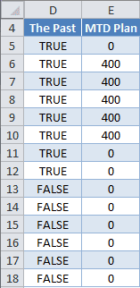
As an introduction to Array formulas, in my last post I added two columns. The multi-cell array formulas for columns D and E are:

{=$A$2>=A5:A18}

{=D5:D18*B5:B18}

Both formulas are entered by selecting their respective ranges, typing in the formula, without curly braces, and using Ctrl+Shift+Enter. Excel provides the curly braces, confirming it’s an array formula.

I didn’t include the current day in my last post, but decided to make a slight change in the column D formula here. (>= instead of >)

In the column D formula, the absolute reference to cell $A$2 could be replaced with the TODAY() function with the same result.

To summarize these two formulas: The Past compares Today’s date to the Date in column A and returns FALSE if the Date is in the future, and TRUE if not.

The MTD Plan multiplies this result times the Plan, and because TRUE = 1 and FALSE = 0, all rows with future date values become zero (0) and otherwise shows the value for the Plan.

A Temporary Single-Cell Array Formula

Summarizing the MTD Plan in a single cell with an array formula will give me a temporary solution for the Cum Plan. In cell B2 I enter the array formula:

{=SUM((D5:D18)*(B5:B18))}

Again, this is done by entering =SUM((D5:D18)*(B5:B18)) and pressing Ctrl+Shift+Enter. Excel provides curly braces.

This formula multiplies together two arrays, then summarizes with the SUM function.

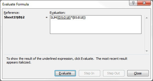
With a single-cell array formula, the Evaluate Formula dialog box allows me to see how this formula is being process by Excel. On the Ribbon, select the Formulas tab, then click Evaluate Formula. In Excel 2003 it’s Tools → Formula Auditing → Evaluate Formula. Excel for Mac doesn’t have this feature.

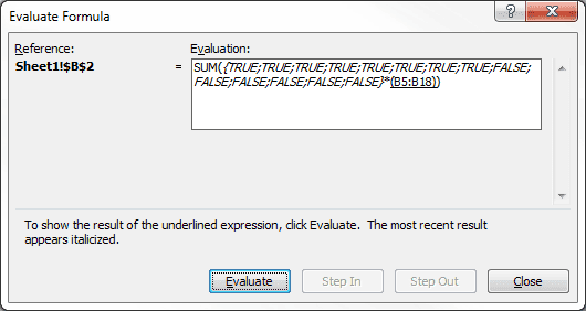
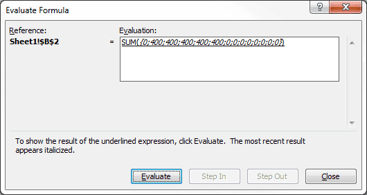
To see the result of the underlined expression, click the Evaluate button. You can see below that D5:D18 is an array that Excel is holding in internal memory. The curly braces are a dead give-away for an array.

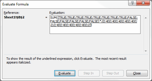
The next time the Evaluate button is clicked, B5:B18 shows up as a second array with numerical values.

Recall from my last post that TRUE = 1 and FALSE = 0. Multiplying these two arrays together gives a single array, which you can see by clicking the Evaluate button again.

The SUM function will now evaluate the array. Clicking Evaluate one more time will show the resulting answer, which is 2000.

My Single-Cell Array Formula

I now want to get rid of columns D and E so all references to them have to be replaced. To edit the single-cell array formula for Cum Plan, I select cell B2, click inside the Formula Bar, replace D5:D18 with $A$2>=A5:A18, then press Ctrl+Shift+Enter to get:

{=SUM(($A$2>=A5:A18)*(B5:B18))}

Since cell A2 contains the TODAY() Function, the following formula works as well:

{=SUM((TODAY()>=A5:A18)*(B5:B18))}

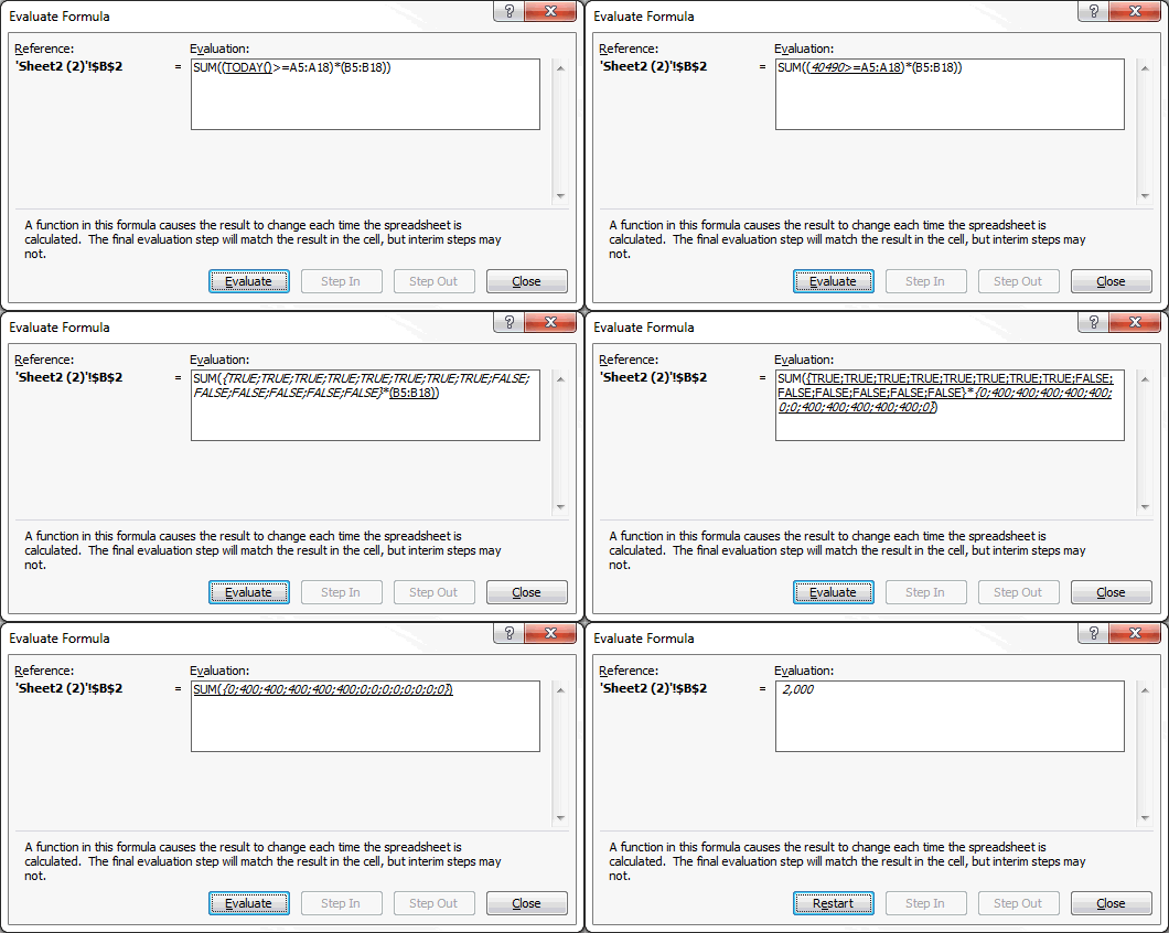
The formula’s calculation progression is similar to the previous screen-shots of the Evaluate Formula dialog box.

The TODAY() Function evaluates to the date serial number 40490, which is November 8, 2010, and is compared to each cell in the array A5:A18 to get an array of TRUE and FALSE values. The second array B5:B18 is expanded to show the numerical values. These two arrays are multiplied together to get a single array of values, which the SUM Function then evaluates and returns the value 2000 to cell B2.

A single-cell array formula can also be applied to the Act Plan for cell C2, which is:

{=SUM((TODAY()>=A5:A18)*(C5:C18))}

And those are my single-cell array formulas.

Note on Excel for Mac

Apparently there is no Evaluate Formula option in Excel 2008 or 2011 for Mac. I have both programs and it simply doesn’t exist. One of the help forum answers suggested using the F9 key, when editing a formula, to show the values in an array, but that doesn’t work for me. back