The INDEX and MATCH functions are used together to perform lookups. The INDEX functions grabs a cell from an array, and the MATCH function contributes the row and/or column position.
INDEX and MATCH Example
Familiarity with the VLOOKUP function can cause you to restrict INDEX and MATCH to less than they can be. The example spreadsheet below bears this out.
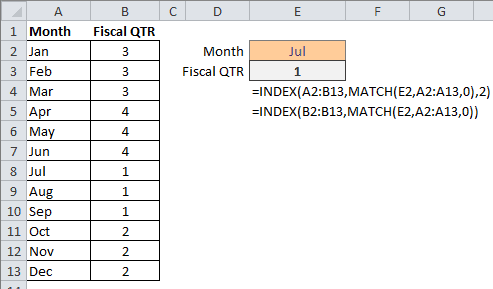
The formula for Fiscal QTR takes the Month in cell E2 as input, finds that value in the Month column, then returns the Fiscal QTR in the same row. The first formula is:
=INDEX(A2:B13,MATCH(E2,A2:A13,0),2)
This INDEX formula uses the array range A2:B13 for the first argument, which is what you may use if familiar with VLOOKUP. But this requires that both the second and third arguments are used (row and column position).
The MATCH function looks to cell E2, finds the exact matching value in the Month range A2:A13, and returns the row number 7 to the INDEX Function for it’s second argument. The number 2 is input for the third (column) argument of the INDEX Function. The INDEX function returns the value 1 from row 7, column 2 of the A2:B13 range.

The second formula:
=INDEX(B2:B13,MATCH(E2,A2:A13,0))
is different in that INDEX uses a one-column range B2:B13, so only a row number argument is required. The MATCH function looks at Jul in cell E2 and finds a match in range A2:A13, returning the number 7 for the INDEX row number argument.
A Grade Lookup Example with INDEX and MATCH
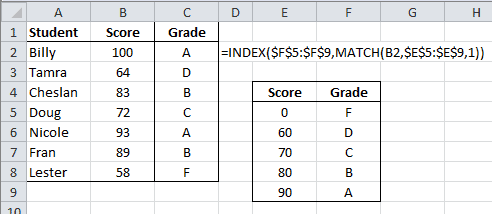
Here’s a student grade lookup formula that relies on the match type argument of the MATCH function to be 1, which finds the largest value, less than or equal to the lookup value.

The formula in cell C2 is:
=INDEX($F$5:$F$9,MATCH(B2,$E$5:$E$9,1))
The INDEX function uses array range F5:F9 and the MATCH function array range is B2:E9. (The dollar signs ($) indicate absolute values because I copy the formula down).
The MATCH function looks to cell B2, which has the value 100, then finds an approximate match of 90 in row 5 in the range E5:E9. The 1 indicates this will be an approximate match. The INDEX function then returns the cell in row 5 of the F5:F9 range, which is the text value A.

Thanks for that, I can’t seem to determine the difference between the following ;
=INDEX(S12 & “”,MATCH(B2,ST_PumpSize,0))
and
=INDEX(Column_C,MATCH(B2,ST_PumpSize,0))
Where S12 = a named range selected on the criteria in B2 & Column_C is a column of data .. is there a reason named ranges can’t be used ? The 2nd one works the first one fails with #Value! .. When I step through the error it successfully replaces S12&”” with Column_C but something then doesn’t work. Any thoughts ?
Cheers,
al.
The INDEX argument requires an Array for the first argument (as you’re using it) so the 1st formula you’ve shown is probably failing in this regard, because of the #Value argument. Perhaps the INDIRECT function might be used to wrap the S12 & “” argument. However I’m not too proficient at using that function.
I have another article that might be of use which looks at a dynamic, dependent drop down list, and uses both INDEX and MATCH in this manner.
Thanks again I’ll have a looksee!
Cheers.
Thanks for the nice article. I can’t seem to make it work though! I try your example and excel says there is an error in the formula. It is getting very frustrating and I can’t figure out what’s wrong with that!!
Leon.
I don’t know what to say, except that I’ll email you the spreadsheet.
I want know about the index match formula how we will use this formula and what is the use of the formula
please tell me
and as per my requst how can we make macro in excel
please rply the excel attachment asap.