The INDEX and MATCH functions working together are more flexible than using the VLOOKUP function. However, if you’ve never used INDEX and MATCH to perform a lookup it can get confusing.
I’m going to cover the INDEX function here so you can learn it well and don’t have to think about it too much when we put it together with the MATCH function.
The INDEX Function Details
The INDEX function returns a cell value from a range, given a row and/or column position number. The syntax is:
INDEX(array, row_num, [column_num])
- Array is required and is a range of cells or an array constant.
- If array contains only one row or column, the corresponding row_num or column_num is optional.
- If array has more than one row and column, and only row_num or column_num is used, INDEX returns an array of the entire row or column in array.
- Row_num is a row number within the array. If omitted, column_num is required.
- Column_num is a column number within the array. If omitted, row_num is required.
If both row_num and column_num are used, INDEX returns the value in the cell at the intersection of the two within the array.
Examples of the INDEX Function
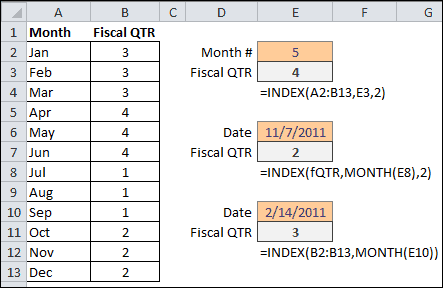
In the spreadsheet examples below, array is the range A2:B13, which is also given the named range of fQTR. The first INDEX formula in cell E4 returns the Fiscal Quarter from the array. The formula is =INDEX(A2:B13,E3,2).
The row_num argument is the Month # in cell E3, which is 5. The column_num argument is 2, and entered directly into the formula. The INDEX function looks to the array, pulls out the value from the cell intersecting the the 5th row and 2nd column, and returns the value 4.

The second INDEX function example in cell E9 uses the named range fQTR for the array. The formula is =INDEX(fQTR,MONTH(E8),2).
The row_number argument uses the MONTH function to pull out the number 11 from the Date in cell E8. The column_num argument is 2 and entered directly in the formula. The INDEX function returns 2 for the Fiscal Quarter, because the 11th month of the Date corresponds to the 11th row and the value in the 2nd column is 2. The value in row 11, column 2, of the fQTR array is 2.
If you wanted to get away from using 2 for the column_num argument, an alternative would be to use COLUMNS(fQTR) or COLUMNS(A2:B13), which would give you the total number of columns or last column in the array range that is 2 in this case. The formula would be =INDEX(fQTR,MONTH(E8),COLUMNS(fQTR)).
In the third example, since each value of Month corresponds to the row number, Jan =1, Feb =2, etc., the INDEX array argument only has to contain the column of data for Fiscal QTR and no column argument is required. The INDEX formula for converting a date to Fiscal QTR is =INDEX(B2:B13,MONTH(E10)).
