In my last post I designed a table and set the cell formatting for the first row of data, which will automatically extend to all new rows of data. The great news is that when I add Conditional Formatting and Data Validation to a Table, they also extended when data is added. But first I want to add a couple of formatting changes to my data entry worksheet.
Table Styles
Changing Table Styles is similar in Excel 2010 ( Windows) and Excel 2011 (Mac) yet the Ribbon is much different. The Mac version has a default Tables tab on the Ribbon. The Windows version only shows the Table Tools tab when a Table is active. The rest of this section deals specifically with Excel 2010, but Mac users can follow along by selecting the Tables tab on the Ribbon.
I decided to change the Table Style because I’m not a fan of the header row with white text.  When you select any cell inside a Table, the Table Tools tab appears on the Ribbon. There’s a Table Styles group that shows a single row of styles in a window on the Ribbon.

On the right there are up and down navigation buttons that allow you to see table styles one-row-at-a-time, which is a big waste of time for me. I click the drop-down button to see an expanded window with lots of Table Styles. As you hover over each Table Style icon, the Table on your worksheet should change its appearance, giving you a preview of what your worksheet data will look like.
If you hover your mouse long enough a tool tip will appear with a Table Style reference. I chose Table Style Medium 23, which gives me black text in the header row.

You can manually change the background color of the header row, which will supersede the Table formatting for any style.
Worksheet Style and Tables
Now that my Table has some nifty formatting, one way to make it “pop” is to remove the ever-present worksheet grid lines. Choose the Page Layout tab on the Ribbon, look for the Sheet Options group, and under Gridlines uncheck View. (Excel for Mac: choose Layout and uncheck Gridlines.)
Another unique fact is that when you scroll down so that the Table header row disappears, the worksheet column letters are replaced by the Table headers.
Of course there’s no word wrap or formatting, but at least you have some idea of what data is contained in each column. I always freeze sheet panes. That way you always see the header row.
Conditional Formatting and Tables
This particular data entry Table records a shift summary for each machine. Meaning there can be mistakes when the summary data is tabulated. One safeguard is to require that Setup, Run and Down Hours equal the Total Hours for the shift. That way errors will get highlighted instead of causing problems later when a report is run.
Select a Table Column
I select the Total Hours data in the Table by moving my mouse to the top of the header cell. When the mouse icon changes to a down arrow, I click once to select the data. (Clicking twice will select the data and the header.)
Use a Custom Formula
Again there are differences between Excel 2010 and 2011 so I’ll give instructions for both.
Excel 2010 (Windows)
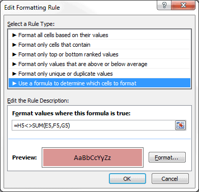
I choose the Home tab on the Ribbon and click Conditional Formatting, select New Rule, then select Rule Type: Use a formula to determine which cells to format. I enter the following formula in the box Format values where this formula is true: =H5<>SUM(E5,F5,G5) then click the Format button and change the background color. Click OK for the changes to take effect.

Excel 2011 (Mac)
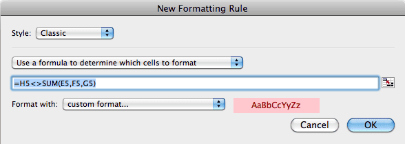
Choose Home > Conditional Formatting > New Rule then select Classic in the drop-down box for Style. Click the second drop-down box and choose: Use a formula to determine which cells to format. Enter =H5<>SUM(E5,F5,G5) in the box for the formula. Select the drop-down list for Format with: and select custom format. Then select Fill, choose a background color and click OK.

Notice the relative nature of the cell references in the formula. This conditional formatting will now extend as the Table expands with more data.

Data Validation and Tables
Data Validation is a great tool to avoid data entry errors. Dates and numbers can offer different problems so I’ll show you a couple different solutions. Remember that when you add more data to a Table the Data Validation extends with each new entry.
Data Validation for Dates
I’ll add some Data Validation to the Date column because Dates are always tricky. Two common data entry errors are 1) hitting the space bar, which results in having a date, that looks like a date, but is really a text value, and 2) missing the slash between month and day, which results in a date that’s in the year 1900.
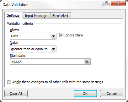
I first select Date column data, then choose the Data tab on the Ribbon, click Data Validation (of Validate on a Mac), and select Data Validation. On the Settings tab, I select Date from the drop-down list, and select greater than or equal to from the Data drop-down list, then finally in the Start Date box I type the formula =$A$5 and click OK.

This will ensure a Date is entered and the value is greater than the first entry. If you aren’t going to enter data chronologically and intend to enter data for previous dates, you can manually type in a Start Date or use a Named Range constant value for the earliest date value likely to be entered into the Table.
Add an Error Alert
After testing this out to see if it works I decide to enter some Error alert text so the user has some kind of idea why they’re getting the message.


