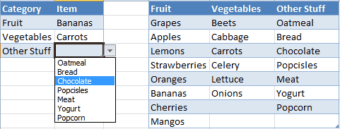
 The other day I was reading a post over at the Contextures blog about Dynamic Dependent Excel Drop Downs and realized that using an Excel Table would provide an alternative method that is both simple and flexible. Tables are available in Excel versions 2007, 2010, and 2011.
In this post I’ll create a Table to hold the Category’s and Items, create three defined names using dynamic formulas, then use Data Validation to create two drop-down lists, the second being dependent upon the first.
Create at Reference Table
Here’s a Table with Category names in the header row and Items in the columns. I just typed in the information then converted to a Table.

Create a Dynamic Defined Name for Category List
Create a defined name for the Table1 Header row range by using the formula =Table1[#Headers]. Please note that Table1 is the name of the Table created in the step above.
This defined name is dynamic, meaning it will expand when more columns are added and shrink if any columns are deleted. It will return the header row of the Table, which we’ll use in the next step. I used myCategory for this defined name.

To create a defined name in Windows choose Formulas > Name Manager then click New…. On a Mac choose Insert > Name > Define…. This will bring up the New Name dialog box that looks like the Edit Name screen-shot shown above.
Create a Category Drop Down List with Data Validation
Type Category in cell A1 for the column heading. Next select cell A2, then choose Data > Data Validation > Data Validation… and in the Data Validation dialog box (shown below) select List from the Allow box, then type in =MyCategory in the Source box, and click OK.
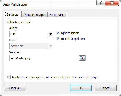
Now cell A2 has a drop down button that shows the Header row of the Table. (Don’t worry about extending this Data Validation down to more rows, we’ll take care of that later.)
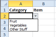
Column B will hold a drop-down list for the Item, which is dependent upon the Category. This takes two defined names to work properly.
Create the First Defined Name for Items
[Update: Select cell B2 before you follow this next step.]
Create a defined name with the following formula:
=INDEX(Table1,0,MATCH(Sheet1!A2,Table1[#Headers],0))
that I’ll name myItemList.
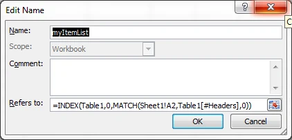
This formula will return a reference to the Table column that matches the Category selection in cell A2 on Sheet1.
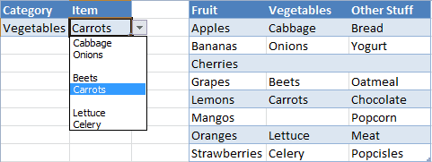
If I use Data Validation to create a drop-down list with the myItemList defined name I’ll get eight items returned because Table1 has eight data rows. As you can see in the picture below, the Vegetables item list has two blank lines, and the Other Stuff item list has one blank line. Not an elegant solution.

However, if you have a table that always has equal items (rows) in each column then this defined name formula will will work well for a Data Validation list.
Create a Second Defined Name for Items
We can create a second defined name that will give us a dynamic list with the exact count. The following OFFSET formula will do the trick.
=OFFSET(myItemList,0,0,COUNTA(myItemList),1)
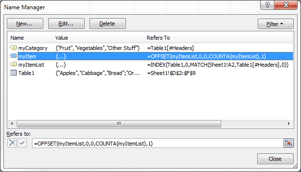
This formula uses the first defined name (myItemList) but alters the height by counting the items. I named this defined name myItem, as you can see below in the Name Manager screen shot.
Create an Item Drop Down List with Data Validation
Type Item in cell B1. Select cell B2 and open the Data Validation dialog box. Choose List and enter the following formula =myItem, then click OK.
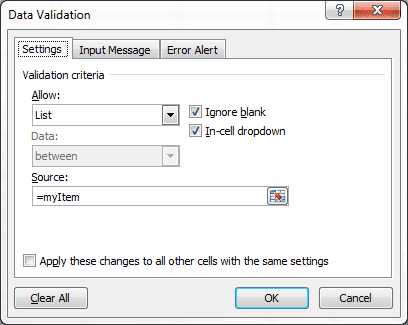
The result is a dynamic drop-down list in the Item column that’s dependent on the Category selection in column A, and returns the exact list.

Convert to a Table
Now it’s time to covert this to a Table, and by doing so the Data Validation will be preserved and automatically expand with the addition of more rows.
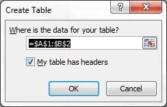
Select cell A2, then in Windows (Excel 2007, 2010) choose Insert > Table, verify the information in the Create Table dialog box, and click OK.
On a Mac (Excel 2011), select cell A2 then choose Tables > New > Insert Table with Headers.
At this point I normally turn off the Data Filter because it’s rather annoying.
As your Table expands, with more rows or columns, this dynamic drop-down list will work just fine. To create a new row in the Table with Data Validation press the Tab key while the active cell is the last column of the last row.
Potential Problem with OFFSET
As you might have guessed the OFFSET formula depends on having items at the top of the list. Should your data have blank rows in the middle of the column, the drop-down won’t have all the items listed yet show blank cells in the list.
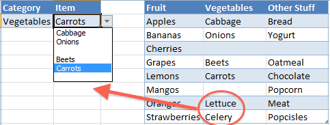
In this case it’s best to use the first defined name (myItemList) in creating a dependent, drop-down list for Item. At least you’ll get all the data, even if it does have some blanks in the list.
Reference Table Location
For illustration purposes I’ve shown the reference Table on the same worksheet as the Category and Item Table. Normally I would place the reference Table on a different worksheet. In this instance none of the formulas would change.

Thanks it is helpfull
hi gregory..i was trying this excercise out and am getting an error message when i put in this Table1[#Headers] . I tried googling but cant figure out any ‘#’ tag functions.
Am lost?
Make sure you have inserted a table into your Excel spreadsheet. Then make sure your table has the name Table1. (You can do this by going to an empty cell and hitting the equals key (=), then selecting the table header.
The resulting formula should be =Table1[#Headers] which you can see in the formula bar. (If you’ve added more than one table, your table might be named Table2). The cell will show #VALUE! because this is and array formula that returns more than one value.
And don’t forget to enter the equals sign when you enter this formula as a defined name (in the Edit Name dialog box).
Thanks greogry!!..it worked.
I had just named it as Table1 and not ‘inserted’ a table as u mentioned.
Very informative, Thanks again!
Glad I could help.
How can I do this with a shared files? Excel Tables are not supported in a Shared Excel File.
@Loretta, you have to replace references to the Table with a range reference. For instance, the top row of the Table, the Header row, can be named myCategory, if defined names are allowed in shared files. Otherwise you can use the range reference D1:F1 where you see myCategory.
Any references to Table1 can be replaced by its range reference, which is D2:F( in this blog article example. The defined name for myItemList would become =INDEX($D$9:$F$9,0,MATCH(Sheet1!A2,$D$1:$F$1,0)) but the problem with this is that the table is not dynamic. If you add data to the table (that’s not a table) you have to change the range reference.
The alternative is to add defined names for the table, in other words create a defined name, like myTable, and give it the range reference of your table range, minus the header. If you want to add data to the table, insert a row between one of existing rows of the table, not at the end, and the table range will automatically resize.
Hi Gregory,
this is an amazing tutorial. Very helpful indeed. I have one question.
In the first dropdown if I change the value, how do i clear out the dependent column – So if I update A2, i want B2 selection to be cleared
thanks
Lalit
@Lalit you can do this with some VBA code in the worksheet. Use the keyboard shortcut ALT+F11 to bring up the VBA Editor. Make sure the Project Explorer is showing (select View > Project Explorer if not showing). Then double-click the sheet with the drop-down list, like Sheet 1. Then at the top left box where is says (General) select the drop-down handle and select Worksheet. Then select the drop-down handle for the top-right box and select Change. Then type in the following code (starting with If Target):
Private Sub Worksheet_Change(ByVal Target As Range)

If Target.Address = Range("A2").Address Then

Range("B2").ClearContents

End If

End Sub
Now every time the contents of cell A2 changes, cell B2 will have its contents cleared.
thanks Gregory,
Appreciate your quick response. This kinda works. Only issue is that B2 gets cleared on select rather than on change. so if i go back to A2, B2 clears even if i haven’t changed the value
You picked Selection_Change instead of Change. I did the same thing at first. Just go to the top right drop-down box and make sure you pick Change, then move the code and delete Selection_Change.
thanks.that worked. Just fyi, to apply this for an entire column, (i.e if i change any item in column B, the corresponding value in C clears), the code looks like
If Target.Column = 2 Then
Target.Offset(0, 1).ClearContents
End If
thanks again
You are a genius. This is the best system for dependent validation lists I have found after countless hours of search.
Wish you a lot of success.
I appreciate the comment.
Hello,
I have following question. Lets say you selected a value in column A, as Fruit, and then in column B you select Banana. Now if you go back to the same row, and you change the selection in column A to Vegetable, in column B you still have Banana. Is there a way around to block the list in column A when there is a value in Column B?
Best regards and thank you for your great solutions!
Yes, but it requires some VBA code. @Lalit had the same question, which I answered and you should be able to review my answer and her response in the comments above.
Dear Gregory,
thank you very much for you help!
Dear Gregory: I have followed the instructions several times but encounter an error when I attempt to set the data validation for the Item B2 cell, I receive the following, “The Source currently evaluates to an error. Do you want to continue?\” Any ideas as to what I am doing incorrectly?
I haven’t seen that error.
Let me find the file I used in the blog post and set it up to be downloaded. This will give you a live example that you can use to compare it to your file. (It might take me a day or so to get this done)
If that doesn’t work you may send me your file so I could take a look and see where the problem resides.
I posted a link to the file, but here’s another link just for you. Let me know if you are not able to fix the “error” you are getting and we’ll figure out what’s wrong.
Hi Gregory:
Thanks again for the quick reply. I still cannot get this to work correctly. Still getting the same message. I am sure my mistake should be obvious but I cannot see it. If I try and insert data valadation in cell B2, I get the same error message – “The Source currently evaluates to an error. Do you want to continue?” However, it worked when I tried it in cell B1, which contains the Header label “Item.” Any ideas?
Same for me. I have tried this numerous times and it looks a great idea but I always get stuck with this same issue and error message – it met be something simple… but inscrutable
The problem that @lisa had was indeed simple. The myItemList formula =INDEX(Table1,0,MATCH(Sheet1!A2,Table1[#Headers],0)) was slightly off. She had typed D2 instead of A2 for the cell reference and that evaluated to an error.
Geezer, were you able to find a solution. I’m getting the same error and can’t find my mistake.
Tx,
If you don’t have anything in the first column selected, your second list won’t work and will get that error – just select some fruit or something in A2 before you go ahead and set up the data validation in B2.
Yes, when there is no selection in the first column, the second column drop-down does not have a reference for the formula. That’s how it’s designed. There are ways around this by writing an IF/THEN statement, which directs the Data Validation to do one thing with a blank cell and another if not.
Great walkthrough – I have one question – Is there any way to create a third tier?
For example – Category Item Make
Fruit Carrotts Asda Carrotts
Sainsburys Carrotts
etc etc
A third tier may be possible, but it makes my head hurt to even think about it. Using the second level column data as the third level column header may be a starting point, but if you have multiple columns on the second level this would mean several third level tables, which means that a single lookup might be difficult, or unworkable unless you use a consolidated range. Now I’m headed for the Tylenol.
Wonderful article! I just applied your process to a third tier. My columns are “Category”, “Type”, and “Subtype”. Table1 has Category for headers and Type for values, and an additional Table2 has Type for headers and Subtype for values. I found I could skip the step of naming the Table2 headers (it’s not needed for data validation of the 2nd tier: that is done with the first table and your original steps.) I repeated the steps to Create a First Defined Name (this time for “mySubtypeList”) and Create a Second Defined Name (this time for “mySubtype”). That final name was used for data validation of the third tier.
That sounds totally awesome! Now if I could just figure it out just exactly what you mean …
I’m trying to follow this, but can’t make it work… it gives me the usual error “The Source currently evaluates to an error. Do you want to continue?\” when doing Data Validation. I tried with all the cells to refer to I can think of bu no change… Anyone can help?
@Renata, go the the bottom of the article where you’ll see a link to “download this file.” Click the link, download the file and see if you can follow what I did. Maybe you can see where your error is located.
@Gregory, thanks. But actually I managed to create the system (and working perfectly) for a second tier, now I need the 3rd thier, like it was explained by the other guy (Steph P). This is the bit that I cannot make it work 🙁 And I need to deliver the file in few hours, argh, “grattacapo” as we would say in italian.
Thanks anyway, and great job, great system, really very useful, thanks Gregory!!
Hi Gregory. Thanks for the great tutorial! I have a question– how would I set up a dynamic dependent drop-down list if I wanted a user to be able to enter any date in the second field column. So, First column has a drop-down menu created from a defined name, and then, based on what value in the defined name is chosen, an answer or a blank cell will appear which can be modified with any date. I get the theory, but not how to put it into practice.
You can’t have it both ways. If you choose a List in the Data Validation dialog box you can get anything from that list, but only that list. If you pick Any Value, then you can enter anything, even a date, but you don’t get anything from a list.
Hello Gregory, thank you for the tutorial.
I think I followed closely the instructions but I get the following behaviour:
regardless of the category I choose, the list in the items drobdown is the firs column of the Table1 (including the header of column 1). I cannot find the mistake.
Thank you
got it – I was mixing some names and, consequently the referenced cells.
Hello;
I notice that when adding a new row to the table you crated, you are still allowed to select the category but not the item, the list for the item is no longer there.
I’m having the same proble with my file, can you help!
Thanks
I’ve had a few people tell me they’ve had some trouble getting all the steps right, so I added an [UPDATE] section to the bottom of the post with a link to the file I used. Please download the file and you can follow what I did, and perhaps see where your work differs.
If you still have issues, please use the Contact page and send me an email. We can figure it out together.
Hello Gregory@
Tried again with the updated link, and recreated my excel file, i’m still getting the same problem…
Please help!
I’m glad I found this. I have been using the dependent drop down validation list, but putting the OFFSET formula into the data validation field, rather than using the table mehtod described above. I was going to convert what I had done using the instructions above. Does it matter if I have created the tables already?
My table is”Equipment”. The column that defines the dependency in Equipment is “Category” and the dependant column is “Model_Name”. Here is what I currently have in the data validation field:
=IF(E2=””,Category_List,INDEX(Category_Column,MATCH(E2,Equipment_Column,0)))
I am defining the “Category_List” as a named range using the offset commands:
=OFFSET(Variables!$A$2,0,0,COUNTA(Variables!$A:$A)-1,1)
I am defining the “Category_Column” as a named range using the offset commands:
=’Equipment Models’!$A:$A
I am defining the “Equipment_Column” as a named range using the offset command:
=’Equipment Models’!$I:$I
Would like to simplify this if at all possible and use the power of the table functionality. Suggestions?
@Trish, based on what you said and what I understand: Your first data validation list would be the defined name myCategory and the formula is =INDEX(Equipment[#Headers]). The second data validation list will be another defined name myItemList and the formula is =INDEX(Equipment,0,MATCH(E2,myCategory,0)). Notice that in this last defined name formulas that I used your reference to E2, and I’m not sure which sheet it’s on. The second thing is that I used myCategory for the MATCH reference, instead of retyping INDEX(Equipment[#Headers]).
Gregory,
I am trying to use the formula….=INDEX(Table1,0,MATCH(Sheet1!A2,Table1[#Headers],0))….in a spreadsheet where I want each row to return a selection made from my table. I have created the table in a seperate sheet and when I use the formula I only get the selection I made in the first row.
My formula is.for a defect type with the name Defect_2 in the name manager..=INDEX(Closed_Lists!$G$2:$L$9,0,MATCH(Tracker_List!$J$11,Closed_Lists!$G$1:$L$1,0))..
The idea being that I select a defect from the table in cell J11 and cell K11 gives me a second list of defect types from the table to choose from. I copy down the formula through the spreadsheet, but can only get the subsequant rows to return based on what is in row 11.
Any help please?
Your formula should work, but it’s an array formula and hence you only see the first cell. Put your formula in a Defined Name, and call it something like myList. Then create a Data Validation list in a cell, and the list is =myList. Then you’ll see the full list from the table.
Gregory,
Does the data validation have to be in every cell in a particular column or just the first one?
I’m not all that good at excel and didn’t fully understand how to do as you suggested.
Could you provide a little more guidance please?
I’m using Data Validation in this example to simply show a list of value in one cell. I wrote an article on Data Validation you can read by clicking this link.
Gregory,
Great tutorial, very helpful. Is there a way though to build the same dynamic dependent lists if the table headers were actually rows and not columns? For example, if the table was set up like this:
category values
———————————-
fruit Grapes
fruit Apples
vegetables Celery
other stuff Bread
other stuff Yogurt
I would still like to have a category drop down, and then based on the category chosen, the values dropdown would only show those associated to the specified category.
Yes, but your table needs to look something like this:
Fruit Grapes Apples
Vegetables Celery Beans
Other Stuff Bread Yogurt
Name the first column myCategoryH in a named range, then define another range name for the rest of the table and call it myTableH.
Next create a defined name myItemListH and the formula will be =INDEX(myTableH,MATCH(Sheet1!D1,myCategoryH,0),0)
The second argument of the INDEX function will get the row match, and putting a zero in the last argument will return the entire row.
In cell A2 set the data validation for a list =myCategoryH, and in cell B2 set the data validation to a list =myItemListH.
Now you have a horizontal lookup.
Gregory,
I really appreciate you sharing the configurations for the dynamic depend list. I have a question I hope you can help me.
I am trying to create a very simple database using the form function from excel. Actually I downloaded the J-walk addin so I can use depended lists for several of the entries. My problems is that when I try to use the dynamic entries for the selection in the form, the list does not come up. But when I try to select the entries on spreadsheet it works fine.
Let me know if you can help me?
Thanks
Monica
I would need to see the spreadsheet and the form to answer your question. I haven’t tried to do any dependent drop-down lists inside a form so I’m not sure how that would work.
Greg,
I created a VBA code using combo boxes to accomplish what I was doing before with the form function in excel. I am able to assign named formulas to the combo boxes, but when I tried to assigned the depend box it does not seem to work.. Have you done dependent drop down list using combo lists in VBA?
Thanks,
Moniac
I have not tried to do this with VBA, but given the amount of interest in this particular topic I might have to do something that will automatically update with VBA. Sorry I’m no help. If you feel comfortable sending my your file, contact me and I’ll take a look.
Gregory,
Thanks. How do I send you a copy of my excell file? I love ot have some help..
Thanks,
Hi Greg,
I have a question. I am trying to create a drop down list where the options in the list show detail but when you select it, the display cell has a concise version of the selection. Is there a way to do this?
I’m not entirely sure I understand the question. What do you mean by “the display cell has a concise version of the selection?”
Hi Greg,
Here is an example of what I mean. In the cell where the drop down list exists. I want the drop down list to have a detailed explanation: eg ‘orange: a citrus fruit’ however once I select that option I want the cell to only show ‘orange’
Thanks again.
I don’t know how to do that in the same cell. Debra Dalgleish has something about doing this very thing on her site, but VBA is involved. I don’t think it’s complicated.
Hi Greg,
I would like to build a spreadsheet that contains a department field. Then Based off of the department field a chart of accounts list will be filtred to the correct accounts for that department and allow multiple entries.
Can you help me with this?
Policy
Etcc…
You could use this article and pretend that Category was the Department, and Accounts was the Item. Multiple entries would have to be in different rows. So instead of Fruit, Vegetables, etc. you would have Dept 1, Dept 2, etc. and then under Dept 1 you would list it’s chart of accounts.
If you’re not sure about this send me an email on the contact page.
I tried creating a data table ,cross checked it points to correct name as Table2.
Also created user defined name in similar to mycategory as DynT2 .
Post this , in another sheet where i want to get this dynamic data tables value , i tried to include this DynT2 into the data validation of the cell .Post this Iam getting only the header values of T2 and nothing more .
I don’t understand why at all we had to create ItemList & Items User defined names and how it is linked to the cells..
I also tried this similar procedure in the same sheet still getting same issue.
can you throw some more light onto this..
If you follow the article exactly it will work. Common problems are missing something simple that you don’t see when you go back and look over what’s been done. That happens to me more times than I like to admit. Try downloading the example file from the article. That will give you a working spreadsheet that you can tinker with and modify.
Hi Greg,
I’m trying to create a conditional drop-down list that contains repetative information. I have 3 columns, one is Office (select the State the office is located), next column is Department (eg Banking, Property) and the third is a list of staff members within that particular office working in the selected department. The departments are repeated for each State an office is located. I’ve been able to set up the first two columns correctly but because the departments are repeated for each State I’m not sure how to populate the appropriate staff members in a drop-down list. If I select the department as “Banking” in one row then the next time I select “Banking” I get the same staff members listed even though the offices are in different States. Just wondering if you can help me this?
Any help would be greatly appreciated.
It sounds like you have to concatenate the State and Department so that you have a unique list for staff members. AK-Banking, CO-Banking, HI-Property, MN-Property, etc.
Hey Gregory,
I know your defintely getting a lot of praise for your brilliance and you deserve it. It took me a while to read through all the interesting comments but I didn’t see my question be asked so here it goes:
Is it possible to choose from the drop down list and instead of filtering the results, display all the results. Here is an example.
If you choose January, on A2, then
…
January 25, 2012
January 26, 2012
January 27, 2012
January 28, 2012
January 29, 2012
January 30, 2012
January 31, 2012 pops up. If we chose February,
February 23, 2012
February 24, 2012
February 25, 2012
February 26, 2012
February 27, 2012
February 28, 2012
February 29, 2012
shows in the same cells as January if I chose that prior.
I didn’t think it was going to be this hard to figure out! Is this even possible on Excel?
Thanks a lot,
Ray
I don’t know how to show the days of the month in the same cell that you choose the month, i.e., cell A2. You can have the days show up as a list in cell B2, but I’m sure you’ve figured that out. Sorry I couldn’t be of more help.
I was able to follow your directions above and successfully create one dropdown based on another on a sample file with Sheet1 as sheet name and using Colunmns A2 and B2 in that sheet but when I tried to adjust so I could use on my Working file and Sheet called external ‘IHD Hiring Sheet’ and Columns F and G, I cant get the second drop down, in column G (based on data in Column F) to work. I am sure I am missing something simply, I hope you can help.
It’s not clear to me what you did to “adjust” the sample file to the working file. It might be best to remove what you have, and start over in your working file. Or you could use the Contact page on this blog and email me a better description of how you made the adjustment, from sample file to working file.
If the working file is something you could share, then we can work out how to get me the file to take a quick look. It’s probably something simple like a range address that is slightly off.
This is a wonderful resource. I’m using it to evaluate my student’s sign language performance. Instead of having to retype the same comments again and again, I put the comments in a drop down. I also put the vocabulary they need in the story in a dropdown, then created columns of error1, error2, etc. with the same vocabulary list copied using a formula. With the vocabulary in a table, I can automatically update it adding new vocabulary.
I just modified it a little to get the student’s names in the first evaluation column, then added the errors in the subsequent columns. It’s set for pivot tables now too.
Thanks a ton!
Hi Greg,
I was looking for a way to provide dropdown values based on a value chosen by the user, and your post has helped me with just what I needed. Thank you for this post, it has been very helpful.
I’ve tried to implement this solution in one of the situations where there are too many categories and few items under each category! So maintaining these categories in a conventional table means several columns with few values under each column. It would be nice if I were to maintain the categories in a single column and list the values for each category in the same row against each of them — simply put, I want to transpose the table values for easy maintenance and still need this solution to work somehow [am I expecting a magic to happen here :|] appreciate any help or assistance you can provide.
Thank you.
Sorry for the delay in responding. I wrote a post on this topic: A Dynamic Dependent Drop Down List with a Horizontal Table Reference. Essentially you can transpose your table values and the category headings will now be row headings in the first column. This means you can’t use an Excel Table because, by default, the headings are in the top row. You can use a named range for the data table and then alter the formulas as I did in the aforementioned post.
Updating the table is a little tricky as you have to be careful to make sure the defined name references the entire table. It won’t automatically update. You have to add data to the table, then update the defined table name so the formulas will work. This can be done with a little VBA, but is probably outside the scope of your original question.