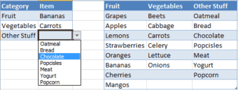
 The other day I was reading a post over at the Contextures blog about Dynamic Dependent Excel Drop Downs and realized that using an Excel Table would provide an alternative method that is both simple and flexible. Tables are available in Excel versions 2007, 2010, and 2011.
In this post I’ll create a Table to hold the Category’s and Items, create three defined names using dynamic formulas, then use Data Validation to create two drop-down lists, the second being dependent upon the first.
Create at Reference Table
Here’s a Table with Category names in the header row and Items in the columns. I just typed in the information then converted to a Table.

Create a Dynamic Defined Name for Category List
Create a defined name for the Table1 Header row range by using the formula =Table1[#Headers]. Please note that Table1 is the name of the Table created in the step above.
This defined name is dynamic, meaning it will expand when more columns are added and shrink if any columns are deleted. It will return the header row of the Table, which we’ll use in the next step. I used myCategory for this defined name.

To create a defined name in Windows choose Formulas > Name Manager then click New…. On a Mac choose Insert > Name > Define…. This will bring up the New Name dialog box that looks like the Edit Name screen-shot shown above.
Create a Category Drop Down List with Data Validation
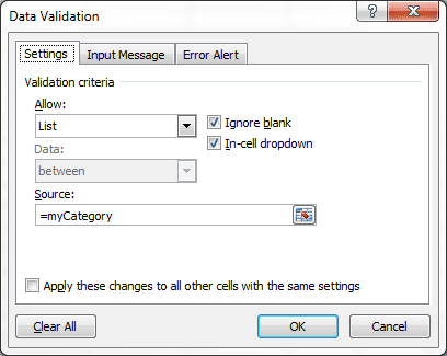
Type Category in cell A1 for the column heading. Next select cell A2, then choose Data > Data Validation > Data Validation… and in the Data Validation dialog box (shown below) select List from the Allow box, then type in =MyCategory in the Source box, and click OK.
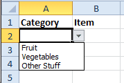
Now cell A2 has a drop down button that shows the Header row of the Table. (Don’t worry about extending this Data Validation down to more rows, we’ll take care of that later.)
Column B will hold a drop-down list for the Item, which is dependent upon the Category. This takes two defined names to work properly.
Create the First Defined Name for Items
[Update: Select cell B2 before you follow this next step.]
Create a defined name with the following formula:
=INDEX(Table1,0,MATCH(Sheet1!A2,Table1[#Headers],0))
that I’ll name myItemList.
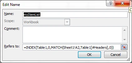
This formula will return a reference to the Table column that matches the Category selection in cell A2 on Sheet1.
If I use Data Validation to create a drop-down list with the myItemList defined name I’ll get eight items returned because Table1 has eight data rows. As you can see in the picture below, the Vegetables item list has two blank lines, and the Other Stuff item list has one blank line. Not an elegant solution.

However, if you have a table that always has equal items (rows) in each column then this defined name formula will will work well for a Data Validation list.
Create a Second Defined Name for Items
We can create a second defined name that will give us a dynamic list with the exact count. The following OFFSET formula will do the trick.
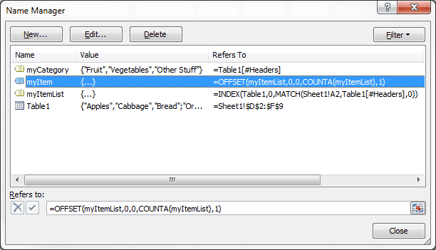
=OFFSET(myItemList,0,0,COUNTA(myItemList),1)
This formula uses the first defined name (myItemList) but alters the height by counting the items. I named this defined name myItem, as you can see below in the Name Manager screen shot.
Create an Item Drop Down List with Data Validation
Type Item in cell B1. Select cell B2 and open the Data Validation dialog box. Choose List and enter the following formula =myItem, then click OK.
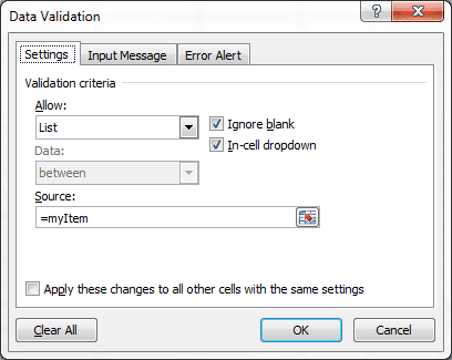
The result is a dynamic drop-down list in the Item column that’s dependent on the Category selection in column A, and returns the exact list.

Convert to a Table
Now it’s time to covert this to a Table, and by doing so the Data Validation will be preserved and automatically expand with the addition of more rows.
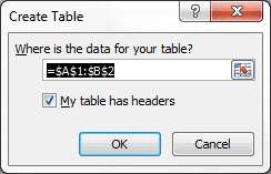
Select cell A2, then in Windows (Excel 2007, 2010) choose Insert > Table, verify the information in the Create Table dialog box, and click OK.
On a Mac (Excel 2011), select cell A2 then choose Tables > New > Insert Table with Headers.
At this point I normally turn off the Data Filter because it’s rather annoying.
As your Table expands, with more rows or columns, this dynamic drop-down list will work just fine. To create a new row in the Table with Data Validation press the Tab key while the active cell is the last column of the last row.
Potential Problem with OFFSET
As you might have guessed the OFFSET formula depends on having items at the top of the list. Should your data have blank rows in the middle of the column, the drop-down won’t have all the items listed yet show blank cells in the list.
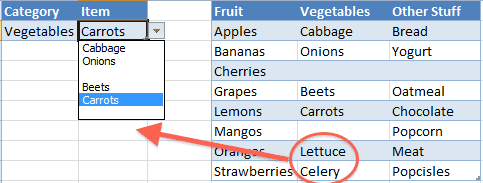
In this case it’s best to use the first defined name (myItemList) in creating a dependent, drop-down list for Item. At least you’ll get all the data, even if it does have some blanks in the list.
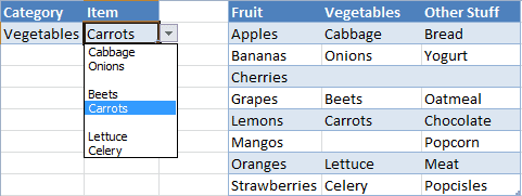
Reference Table Location
For illustration purposes I’ve shown the reference Table on the same worksheet as the Category and Item Table. Normally I would place the reference Table on a different worksheet. In this instance none of the formulas would change.

Hi Gregory! Really helpful tutorial
I just have one question, when you are creating the Defined Names for ITEMS are you selecting the whole table when defining the name or just the items without the headers?
Thanks!
Sorry! I figured it out, it was not like that at all..
And again thanks a lot for the tutorial, really helpful!
Thanks for the compliment, and I’m glad you figured it out.
This has worked fantastically for me, thanks.
I am having one problem though, where I’m trying to make the dependent list across 3 columns, the data validation says that “The Source currently evaluates to an error” and the drop down does not appear on any column but the first one.
Any ideas?
Possible reasons for the error:
– There is an error in your formula.
– When you set up the defined range formula for the third column, you didn’t have the first cell selected, which throws off the relative reference.
– Your formula is an absolute reference instead of a relative reference. ($C$2 instead of C2)
Hope that helps.
Hi Gregory
Many thanks for an very useful guide – unfortunately I also get stuck with the same error message as with Cameron. I suspect that it has something do with the naming of the items (one previous comment mentioned that she “figured it out” – unfortunately she did not elaborate).
It would be very helpful if you could clarify the following:
1. Do you select all items when naming them?
2. In your file – how come you refer myItemList to C2 (an empty cell)?
3. My “table” contains filers on top – not sure if this can be a problem?
Many thanks,
Viktor
1. The only cell I selected when creating a defined name was myItemList. And that cell was B2. The reason is the formula in this defined name will reference the cell immediately to the left of the active cell. So you have to select the correct cell and then change the absolute reference to a relative reference, meaning the $A$2 is changed to A2. This allows the formula to be copied down and each reference will be to the cell immediately to the left.
The tables create their names automatically. The other defined names, myCategory and myItem were just typed in because there was no cell or range reference.
The only time I select all the cells is when I create a defined name for a range.
2. If you select cell B2 and then choose Insert > Name > Define and select myItemList, you will see a reference to A2. If you select cell D2 and do the same thing, you will see the cell reference is C2, which happens to be the cell to the immediate left. So myItemList will show the cell to the immediate left of the active cell.
3. The Table filters aren’t a technical problem, everything will work fine with the filters on. However in this instance I don’t care for them because they get in the way of reading the column headings and they aren’t used. So I turn the filters off by choosing Data > Filter.
Hope this helps.
I am having one problem though, where I’m trying to make the dependent list in first column, the data validation says that “The Source currently evaluates to an error” and the drop down does not appear on any column. Gregory started with third column, but I happen when the first column.
Gregory,
I found my problem, thanks, very helpful.
Best tutorial on the subject! Thanks!
However, I really struggled to make this “dynamic” to an entire column. Meaning: $A$1 limits the drop-down options for $B:$B. Your examples always include a single-cell reference for the MATCH value (“MATCH(Sheet1:A2”) but I really wanted to have $A$1 limit the drop-down for $B$1 and $A$2 limit the drop-down for $B$2 and so on.
I first tried to replace your single-cell reference with a named range reference (“CategoryCol”), but no such luck.
Then I realized I needed to have the formula first reference the specific cell I wanted to match. I was able to adjust my formula to create dynamic drop-downs in the spreadsheet columns that are relationally connected to the “parent” column on a row-by-row basis.
Example:
=INDEX(Table1,0,MATCH(INDIRECT(ADDRESS(CELL(“row”),COLUMN(CategoryCol))),Table1[#Headers],0))
However, with your mad skills, I’m wondering if there is a simpler, more stable solution than the one I found?
The single cell reference is designed to be relative. Meaning that I select cell B2 and create the myItemList defined name and refer to cell A2. If $A$2 is the reference then the formula will only reference the first cell. By using a relative reference, A2, the myItemList always refers to the cell just to the left of the active cell. Therefore it can be copied down column B and it will work perfectly.
The key is to create the relative cell reference in the first row while the active cell is B2, and the reference is cell A2. Once this is done your set.
Thanks, Gregory. That does make sense. I did re-try your sugtion to create a simpler formula. I couldn’t apply this validation rule to the entire column successfully, which is a key for me since I can’t predict the number of rows that will ultimately be used. However, I also cannot turn the dynamic drop down sheet into a table, which I think you said would maintain the validation. My formula, while clunky, does handle these restrictions. Thanks again. You let me impress my boss with my semi-pro skills!
If you put your reference table on a different sheet and give it a defined name, you can have the range name automatically update with some easy VBA code. I wrote a simple post to cover this technique.
Nice tutorial.
I used to take advantage of pivottables to dynamically get the content of my named range since PT can give sorted lists without duplicates and without blanks (offset and countA the PT list as final).
The workaround was to trigger my RowField everytime an item was choosen in, say listbox_1 to get the dynamic contents list ot that item in, say listbox_2.
Always good to learn new methodes that can do the same job 🙂
I’m having a little weird behavior with this. I have adapted this to a workbook I have, with the table headers Expenses and the items underneath are SubCategories for the Expenses. I have used ExpenseList as the defined name with the INDEX formula, and ExnenseListSub as the defined name with the OFFSET formula. My primary validation is in column D, starting on cell D68. I’ve noticed that when I choose something in cell D68 from the validation list, the ExpenseList formula changes to something funny, like =INDEX(Table1,0,MATCH(AUG!$D104954,Table1[#Headers],0)). AUG!$D104954 is not in the range I want to use for the table, which should only go from row 68 (67 with headers) to around row 225, will probably never need more than that.
Any clue why this is changing?
Thinking about it, I looked at the example provided in this post, and saw the same thing happening. In the defined name myItemList, A2 is changing to some whacky cell, such as XFD2, so the formula reads =INDEX(Table1,0,MATCH(Sheet1!XFD2,Table1[#Headers],0)).
I just noticed, the INDEX formula AUG!$D#### is changing to whichever cell I have currently selected in column D, as long as only the column is a fixed value. I made it relative, and it changes to wherever I have the currently selected cell, and sometimes changes to the last possible row (100454095 or something like that) or the last column possible.
Hopefully my previous response to your earlier comment will explain everything.
The main problem is when you create the myItemList defined name formula, which is =INDEX(Table1,0,MATCH(Sheet1!A2,Table1[#Headers],0)) in my example, the Active cell must be where the first formula will appear. In my example, when I created this formula the active cell was B2.
After this is done, your formula will work correctly. The reference in this defined name formula is cell A2, but that is misleading because the reference is relative, meaning that it will always refer to the cell just to the left of the active cell. If the active cell is D30, and you take a peek at the defined name formula, you will see a reference to cell D29.
Similarly when the active cell is in the first column, say cell A68, then the reference will be to cell XFD68, which is the last cell in the same row. The reference wraps back around, so to speak.
Now if you create this defined name formula, for instance when the active cell is cell C20, and you use the same A2 cell reference, then the defined name will always refer to the cell that is two columns to the left and eighteen rows above it. If you then use that defined name formula in cell B2, then you’ll get a reference that is near the bottom, right area of the entire worksheet, because the reference will “wrap back around.”
So you should use an active cell in row 68, where ever you are going to use the formula, then open the myItemList defined name formula and change the cell reference to the proper column where your data is and then the cell reference will work all the way down to the end of the last row. And example would be that the data is in cell D68 and you want the formula in cell E68. Then select cell E68, open the defined name formula myItemList and change the cell reference to cell D68. Then you’re good to go.
Hopefully that helps.
Hi Gregory,
i am using excel 2010 and trying to figure out if the following scenario is possible; any feedback is appreciated..
if i have 5 line items for example that their data is dependent on me choosing a reference (number or letter) from a drop down menu; when choosing the reference (number or letter), is there any way that the cells take the value of the reference from a range that i pre set?
ill try to explain below:
A1 = blank
A5 = blank
A9 = blank
A22 = blank
A71 = blank
my control drop down menu is the following: AA, A, B & C. The data range for those is AA=50, A=100, B=250 and C=500
if i click on B from the drop down menu, (think of it as a legend) i would like for A1, A5, A9, A22 and A71 to all have the value 250.
thanks!
Yes there is a solution. Here’s how I did it. In cell C2 add a Data Validation List by typing in AA, A, B, C. Create a defined name of that cell called myDropDown.
Next enter a lookup table with the same list and their corresponding values. Cell E2 = AA, cell F2 = 50, cell E3 = A, cell F3 = 100, cell E4 = B, cell F4 = 250, cell E5 = C, and cell F5 = 500. Create a defined name for the range E2:F5 with the name myLookup.
Next enter the following formula in cell A1
=IF(myDropDown=””,””,VLOOKUP(myDropDown,myLookup,2,FALSE))
and then copy this formula to cells A5, A9, A22, and A71.
Now when you select a value from cell C2 from the drop-down data validation list, the formula looks at the list value (AA, A, B, or C), looks up the corresponding value, and returns the result to all those cells.
Hi Gregory,
Just wanted to say thank you; worked perfectly!!
Thanks for taking the time and even sending me an excel sheet – much appreciated.
Hi Gregory,
Thank you for your article – I’ve successfully applied it. However, I need to create a third column, which is dependent on the second column (itself dependent on the first column).
The trick is, for column 3 I want to reference a new table, of whose name matches the value in column 2.
I.e. I want to replace “Table1” in the below formula with the value of the adjacent cell in the previous column, in an effort to reference the appropriate table.
=INDEX(Table1,0,MATCH(Sheet1!A2,Table1[#Headers],0))
Does this make sense?
Thank you in advance!
If you want a third column then create a Table2 by using all the data values in Table1 as the Header row. Then fill in the data in Table2.
Next, while the active cell is C2 create a defined name formula, call it myItem2 and the formula is =INDEX(Table2,0,MATCH(Sheet1!B2,Table2[#Headers],0)).
Now create a Data Validation list in cell C2 that is =myItem2.
Hope that helps.
Hi Gregory,
Rather than place all data values of table1 into the headers of table2, I want to break it down with a separate table for each header in table1.
Thanks
Hello,
I’m trying to avoid using the =OFFSET formula because of its volatility.
I have a worksheet that uses the original Contextures solution, but when I change data in a Date cell elsewhere on the same spreadsheet, Excel crashes. I know it’s the Index-dependent lists that are causing Excel to crash because when I disable the “Counter” named range, my spreadsheet no longer crashes when I change the date cell.
Has anyone else encountered a crashing problem with the Contextures method? Does anyone have a solution to the problem?
Thanks,
Elliot
Hi,
Have been tasked to create a database of suppliers globally, by my company. Each company contains 4x fields and the premise of the document is whether the company provides a service in that city. The geographical hierarchy is as follows Region, Country, City.
What I want is to be able to have separate drop down filters for EMEA, Americas, AsiaPac and a static list of suppliers but be able to select different countries/cities and see who from the entire list provides services there.
Really appreciate some advice how to set that up, 1x line example of basic information is listed below.
Algeria Angola
Alger Aberdeen
AECOM http://www.aecom.com Key contact Email Address Y Y
Thanks,
Hunter
These complicated examples are a little hard to visualize when not viewed in a spreadsheet and the description very precise and detailed. Perhaps you could send me an email from my Contact page. I’ll respond and you can send me an example worksheet. I’m not getting the full picture here so it’s hard to point you anywhere, much less in the right direction.
Oops, example didn’t come out very clearly, example below for
EMEA Americas
Algeria America
Alger New York
AECOM http://www.aecom.com Key contact Email Address Y Y
hi…
i have a table of contracts, with the columns contract number, name, state…. in the same file, a different sheet was created in order to apply payments to the contract, i used a drop down list in the cell where i can select the contract number, based on the contracts table previously created; i have to insert rows for every payment made… sometimes there are different contracts for the same providor, so i want to be able to display only the contracts that the selected providor have, as per the contracts table…is there a way to do this using just one table (contracts)?
Your example is a bit confusing. You want to reference a provider, which may have more than one contract, but you don’t list provider in the table of contracts. And when you say you are “inserting rows for every payment” are you really inserting rows or adding different records for the same provider? I don’t really understand the question here. If I would take a guess, on displaying only the contracts for each provider, that would take an Array formula and a (variable) number of cells to return that information. Not really my speciality.
let me try to explain it…
sheet 1:
(a1)contract number (b1)provider (c1)contract amount
(a2)101 (b2)company 1 (c2)$10,000
(a3)102 (b3)company 2 (c3)$5,000
(a4)103 (b4)company 3 (c4)$4,000
(a5)104 (b5)company 1 (c5)$3,000
sheet 2:
(a1)provider (b1)contract number (c1)payment
(a2)*validation data list from the contract names of the sheet 1 (no problem doing this list)* (b2)*here is what i need help for, I need to create another list which displays only the different contract numbers that the providor chosen in the cell a2, has in the whole base of the sheet 1, so do not need to write the whole contract number that can cause a misswriting data and, therefore, can´t get the report of how much have been paid to that particular providor (I am talking about 600+ contracts with around 350+ different providors); in other words, if I choose in cell (a2) the option “company 1”, in the list of the cell (b2)should only show the contract numbers “101” and “104” only… so I can register in the cell (c2) the payment made to that providor for that specific contract (it could be lots of payments for each contract)…therefore, the list of payments of this sheet 2 will be long based on the different payments made to the whole list of contracts…
is there a formula or a way to do this avoiding any script, will be great…
thanks for any advice
This one is beyond me, formula wise. I would resort to some type of programming to see if that would work, but I’m having trouble seeing the solution.
I’ve read through the comments, but something still isn’t working for me…I actually copied and pasted your formulas as stated herein, so I know there are no formula issues. I get my first dropdown in just fine, but the second one won’t work at all. I’m using the defined name “Customer2” for the second dropdown when I do the data validation. I have the following reference for “Customer2”:
=INDEX(Table1,0,MATCH(Sheet1!A3,Table1[#Headers],0))
Where Sheet 1, cell A3 is the location of the first drop-down entry upon which the second is dependent (I have my Table1 in Sheet 2). I have no idea why my second drop-down isn’t working…any thoughts would be much appreciated!
When you create the define name formula for Customer2, the active cell must be where the formula will return the first answer. For example, cell B3 might be where you would want the second drop-down list so that is the active cell where you would create the Customer2 defined name formula.
The formula is actually a relative reference, meaning that, in this example, it will always look one cell to the left for the input.
I thought I’d already tried that, but I just did it again, and voila! One of those things where I think I looked at it/tried too long…I’m an idiot – thanks for the quick response!
Thanks a lot. It’s very helpful even I’ve just used from your sharing a bit.
Hi
This has been a really helpful tutorial for me, i have applied it to some inventory data that i want to use to populate a schedule of quantities from. I have three levels of selection criteria (Category, Type, Size) on approx 1600 different items. My data is ordered by category then type then size.
Category Type Size
widget WA 100
widget WB 150
sprocket SA 50
sprocket SA 60
sprocket SB 50
Sprocket SC 60
To make this work i created two look-up tables on separate worksheets to generate the dynamic drop-down lists:
One sheet with part categories as header with the unique part types listed beneath:
Widget Sprocket
WA SA
WB SB
SC
A second one with part types as headers with unique sizes listed beneath
WA WB SA SB SC
100 150 50 60 50
60
I used Index formulas to populate the look-up tables from. However with 20 categories and over 200 part types the sheet crashes every time i recalculate – frustrating!
Is there a way to create a dynamic drop down list directly from a database listed as above?
Thanks
Jennifer
So far as I know, Data Validation won’t accept the complicated INDEX formula directly, hence the use of the Defined Name formula.
Have you tried leaving your worksheet on auto calculate? Or does that slow it down too much?
Sorry I’m not much help.
Thanks,
I seem to have got it working, by using index and offset formulas in the defined names to reference a unique name lookup sheet, then return data from the original database.
Jennifer
Fantastic! I’m glad you were able to figure it out.
Is there a simple way to save the selections made on sheet 2?
My use case is that I have a table and I want to know how many times Johnny selects the combination of other stuff popcorn vs fruit grapes?
Not that I’m aware of. Sorry!
Dear Gregory,
I like this work alot! Now I want to make it even more dynamic and a new table. So first you choose in a dropdown the main course of the starter. Then from that choice the formula’s get the info from Table1 of Table2.
With indirect I made the choice for selecting the table, but I got a #ref. It looks like =INDIRECT(‘Table’&A1) does not work (indirect and dynamic names bug??). Can you please advise?
If you follow the post closely it should work correctly. You may be missing something simple, so my recommendation is to download the example file at the end of the article and see how I’ve done things, and then compare that to what you are doing.
Thanks for great info. I expect what I am asking is not possible without VBA, but going to ask just in case. How about creating the dynamic lookup from a single table with the first key being a value. For example, a single table of expense codes like travel, training, registration fees, Bank Fees, Interest Income, etc and a second column for each entry indicating income or expense. I would like to be able to select income or expense from a simple drop down (easy) and then have a second drop down populate with only the appropriate choices (harder). The key is the feed data is provided in a single table, and is updated from time to time. I went through the hassle of separating into two separate tables as necessary for this method, and even some VBA to do this automatically when requested, but it would be much easier and simpler to be able to pull the lists from the original table.
The data for the data validation drop-down list does come from a single table. Not sure exactly what you are referring to there.
For your example you would have a two-column table. The heading on the first column would be Income, with appropriate choices in the rows below. The second column of the table would have the heading of Expense, and have a similar list of choices for expenses below the heading. This table could be used to create data validation cell to select the Income or Expense, and then a second cell to dynamically make a selection.
Hope this helps.
Yes, I wondered if I was clear on my question. The data for the lists is provided in a slightly different form. The first column of the table contains ALL the categories. The second column contains the word inc, exp, or memo for each record, and then a third column with either active or inactive. This is not my design choice, this is the way the categories are provided to me. They are updated on a monthly basis.
I have converted this to a table like suggested, with the first column containing only active expense tags, and the second only active income, and the third any memo tags. Works fantastic, but wanted to eliminate the monthly table conversion.
I was hoping someone had an idea how to do this without converting the source table format, and without using vba.
I have successfully created dependent menu lists using the methodology on Contextures. It works great with one exception…it does not process well backwards. For example, in the first menu I select a Region (North America, South America, Europe, etc.). the second menu, which is dependent on the fiorst menu is country (USA, Canada, Mexico, France, Germany etc. and the third is city. Everything works perfectly except if I selected North America and then USA and then Boston and then decided to change the region to Europe the second and third menu selections stay as previously selected…which could lead to an incorrect reporting result. I would like for it to default to being blank when one menu is not possible given the selection of another menu. Any ideas? Thank you, Kurt.
You could change the defined name formula to include an IF statement that looks to see if the reference cell is blank and returns a blank cell, otherwise does the lookup. Something like this: =IF(B5=””,””,VLOOKUP(B5,myVendors,2,FALSE)).
Thanks for the tutorial, Gregory!
One question. Is there a way to clear out the value on the Item (second column) when I select a different Category (first column)? In other words, if I originally selected Fruits as the Category and Bananas as the Item, and then I change the Category to Vegetables (on the same row), can Bananas be cleared out since Bananas are not Vegetables?
You might change the myItemList defined name formula to:
=IF(Sheet1!A2=””,””,INDEX(Table1,0,MATCH(Sheet1!A2,Table1[#Headers],0)))
and see if that works. The formula returns a blank if the reference cell is blank, and otherwise does the lookup.
Hey Gregory,
Thanks for the info..it helped me a lot..
Is there an option for adding the check box function also in the dependent list.
For selecting multiple values from the drop down.
Abhijeet
For a check box option you would have to go with VBA.
Gregory,
Thank you for providing this tutorial. I have one problem though. I’ve created the dynamic list you provided in the example above, works great. However, my problem is that if I were to select “Fruit” as the category first, then selected “Banana” as the type, I can go back and then change my category from “Fruit” to “Vegetables”, thus showing “Vegetables” as the Category and “Bananas” as the type. This is obviously not a valid combination. Is there a way to have the user select only valid combinations regardless of which box is selected first (i.e. if I select “Bananas” in the second box, the only choice I have for the first box is “Fruit”)? Any help on this is greatly appreciated.
I ran into the same error many others have, and one that you have addressed: “The Source currently evaluates to an error” – In general your instructions skip major parts of the building this model. i.e. What cells do you highlight when you create a “Data Validation” versus a “Defined Name”? –
Thanks for all the free instruction though.