How to Add Freeze Panes to the Quick Access Toolbar in Excel

To add Freeze Panes to Excel's Quick Access Toolbar on Windows, open the View tab, right-click the Freeze Panes button, and choose Add to Quick Access Toolbar. The toolbar button opens the freeze options without requiring you to switch back to View each time.

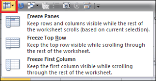
Back in Excel 2007 and 2010, I had recommended adding the standard Freeze Panes command to the toolbar. Then I found a small annoyance: it still took two clicks. One opened the menu; the second chose Freeze Panes, Freeze Top Row, or Freeze First Column. I only wanted Freeze Panes. So why did I have to click twice?

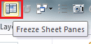
As it turned out, I didn't. A separate command named Freeze Sheet Panes applied the action in one click. It was conveniently hidden from the Ribbon.

That discovery is the original Excel 2007/2010 tip below. The current standard menu setup follows it; availability of the old command name in current Microsoft 365 builds has not been verified.

Add the one-click command in Excel 2007 or 2010

In these Windows versions, the original shortcut used a command hidden from the Ribbon:

1. Right-click the Ribbon and choose Customize Quick Access Toolbar.
2. In Choose commands from, select Commands Not in the Ribbon.
3. Scroll to Freeze Sheet Panes. If you cannot find it, try All Commands.
4. Select the command and click Add.
5. In the right-hand list, use the arrows to place it where you want it on the toolbar.
6. Click OK.

Once added, select the appropriate cell in your worksheet and click Freeze Sheet Panes to apply the freeze directly. The cell selection determines which rows and columns remain visible.

Here is the standard button I had originally recommended. One click opens this menu, and another chooses the action—the extra click I wanted to avoid.

My complaint in 2011 was simple: Excel should have made the one-click action a primary command when the Ribbon arrived in Excel 2007. It was a useful shortcut to leave hidden.

Add the standard Freeze Panes menu in current Excel for Windows

For current desktop Excel, start with the standard command on the Ribbon:

1. Open View.
2. Right-click the Freeze Panes button and choose Add to Quick Access Toolbar.
3. If the toolbar is hidden, right-click the Ribbon and choose Show Quick Access Toolbar.

This uses Microsoft's documented method for customizing the Quick Access Toolbar. The resulting button opens the freeze menu, so you still choose an option after clicking it.

To look for commands that are absent from the Ribbon, open Customize Quick Access Toolbar > More Commands and check Commands Not in the Ribbon, then All Commands. Microsoft's current documentation describes this search method but does not confirm the exact legacy Freeze Sheet Panes command. If that name is missing, use the standard menu or View > Freeze Panes.

Select the cell before freezing panes

For the general Freeze Panes action, select a cell below the rows and to the right of the columns you want to keep visible. Freezing affects the worksheet view while you scroll; it does not prevent you from editing those cells.

For example, suppose row 1 contains headings and columns A:B contain identifiers:

1. Scroll to the top-left of the worksheet.
2. Select C2.
3. Click the historical Freeze Sheet Panes button, or open the standard toolbar menu and choose Freeze Panes.
4. Scroll down and right. Row 1 and columns A:B stay visible.

This follows Microsoft's rule for freezing rows and columns: the rows above and columns to the left of the selection remain in place. For more examples involving both directions, see how to freeze cells so rows and columns stay visible.

The standard menu also offers Freeze Top Row and Freeze First Column. Start at the top-left of the sheet and use those for row 1 or column A alone. To keep several heading rows visible, select a cell in column A immediately below the last heading row and use Freeze Panes. Our guide to freezing a row in Excel covers row-specific examples.

To remove an existing freeze, choose View > Freeze Panes > Unfreeze Panes. Unfreeze first if you need to move the boundary, then select the new cell and freeze again.

If the button is missing or behaves differently

• It opens a menu instead of freezing immediately: you added the standard Freeze Panes command. That is expected; the historical one-click command was named Freeze Sheet Panes.
• Freeze Sheet Panes is absent from the command list: check All Commands, then use the standard menu if it is still missing. The old screenshots do not establish availability in your current Excel build.
• The toolbar is not visible: in current Windows desktop Excel, right-click the Ribbon and select Show Quick Access Toolbar.
• The wrong rows or columns stay visible: unfreeze, return to the top-left of the sheet, and select the cell below and right of the intended boundary before freezing again.

Excel for Mac and Excel for the web

The toolbar instructions above are for Windows desktop Excel. On a Mac, use the Freeze buttons on View; Microsoft's Excel for Mac instructions also say to select View > Normal if the Freeze buttons are grayed out. The Windows screenshots do not describe the Mac toolbar layout.

In Excel for the web, use the freeze controls on View. The historical Windows toolbar customization procedure is a desktop workflow, so do not expect the same Freeze Sheet Panes command list in the browser.