Your PivotTable has the sales figures, but you want the monthly report to keep its own layout. Use GETPIVOTDATA to ask for a figure by its field and item names, such as revenue for East. The report can stay in the same cells while you rearrange the PivotTable.
We'll put a region name in Report!B4 and its revenue in B6. East should return 200, West 100, and North 0. That last result matters: North has actual zero-value records, which is different from a region the PivotTable can't show.
Download the GETPIVOTDATA example workbook. It opens with East selected, revenue of 200, and total revenue of 300. The Sales, Pivot, and Report sheets contain the example below; Notes has reset instructions. The screenshots show Excel for Mac.
Start with an actual PivotTable
GETPIVOTDATA needs an Excel PivotTable. A range of typed totals, a pasted copy of a PivotTable, or a summary produced by PIVOTBY isn't the same object, even if the cells look alike.
To build the example yourself, create three sheets named Sales, Pivot, and Report. On Sales, enter the following data in A4:C10, including the headers in row 4:
| Region | Product | Revenue |
|---|---|---|
| East | Bags | 120 |
| East | Boxes | 80 |
| West | Bags | 75 |
| West | Boxes | 25 |
| North | Bags | 0 |
| North | Boxes | 0 |
Select A4:C10, use Insert > Table, and confirm that the table has headers. Name the table SalesData. Then insert a PivotTable from SalesData on the existing Pivot sheet, starting at A4. If creating the object is new to you, our PivotTable introduction covers the setup.
Arrange the fields like this:
- Rows: Region
- Columns: Product
- Values: Revenue, summarized by Sum
Keep row and column grand totals enabled, and leave every region and product visible. The expected figures are:
| Region | Bags | Boxes | Grand Total |
|---|---|---|---|
| East | 120 | 80 | 200 |
| North | 0 | 0 | 0 |
| West | 75 | 25 | 100 |
| Grand Total | 195 | 105 | 300 |
Check the Values field before continuing. It should say Sum of Revenue, not Count of Revenue. We're adding the amounts, not counting the records. Also check that Pivot!A4 belongs to the PivotTable; the report formula will use that cell to identify it.
Pull East's revenue into the report
On Report, set up these cells:
| Cell | Enter |
|---|---|
| A4 | Region |
| B4 | East |
| A6 | Revenue |
| A7 | Total revenue |
You can let Excel write the first formula by selecting the figure you want. In the example workbook's original PivotTable layout:
- Select Report!B6 and type
=. - Select the Pivot sheet, then click D6, East's grand total of 200.
- Press Return to finish the formula.
Excel for Mac generated this formula for that selection:
=GETPIVOTDATA("Revenue",Pivot!$A$4,"Region","East")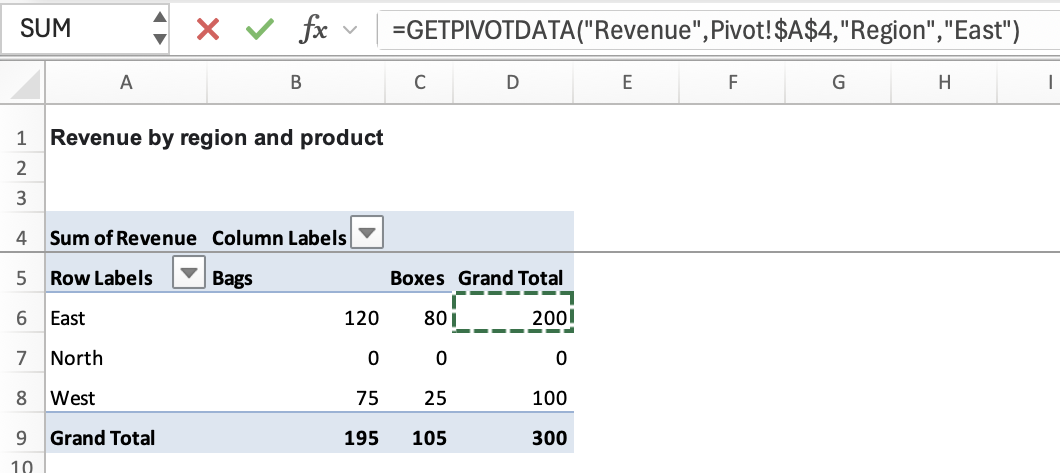
The generated formula asks for East directly. To make the report respond to the region in B4, replace "East" with B4. The workbook's report also uses the full Values caption, "Sum of Revenue", in place of the shorter "Revenue". Both identify the same measure here.
Enter the complete formula below in B6. You can use this manual route from the start if clicking the PivotTable gives you an ordinary cell reference:
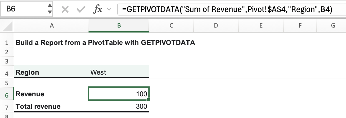
=GETPIVOTDATA("Sum of Revenue",Pivot!$A$4,"Region",B4)The expected result is 200: East's 120 for Bags plus 80 for Boxes.
Follow East through the formula. B4 supplies the item name, East. "Region" tells Excel which field that item belongs to. "Sum of Revenue" selects the amount we want, and Pivot!$A$4 identifies the PivotTable that contains it. We haven't specified a Product, so the request covers East's total across the visible products.
The dollar signs keep the PivotTable anchor fixed if you copy the formula. They don't turn A4 into the result cell: A4 only needs to remain inside the correct PivotTable.
The first argument uses the Values caption in this example. Microsoft also documents using the underlying field name, such as "Revenue", in place of "Sum of Revenue". If your PivotTable uses a custom caption, check the actual field rather than copying a caption from another workbook. See Microsoft's GETPIVOTDATA documentation for the argument rules.
Now enter the grand-total check in B7:
=GETPIVOTDATA("Sum of Revenue",Pivot!$A$4)With all items visible, the expected result is 300. Leaving out the Region/item pair asks for the total instead of one region.
Change the region without editing the formula
Replace East in B4 with West. The same B6 formula should return 100, made up of 75 for Bags and 25 for Boxes. Try North next; its two zero-value records should produce 0.
| Report!B4 | Expected Report!B6 | Expected Report!B7 |
|---|---|---|
| East | 200 | 300 |
| West | 100 | 300 |
| North | 0 | 300 |
B4 selects what the report asks for. It doesn't filter the PivotTable, so the grand-total formula in B7 still covers all three regions.
Keep B4 outside quotation marks in the formula. Writing "B4" would ask for a region literally named B4 rather than reading the cell's contents. Similarly, don't replace the reference with "East" if you want the report to respond when you change the region.
Rearrange the PivotTable and keep the report in place
Make a copy of the workbook for this check, and set Report!B4 to West. In the PivotTable field list, move Region to Columns and Product to Rows. Keep grand totals enabled and A4 inside the PivotTable.
West's figures now run down a product column instead of across a region row. The request in Report!B6 hasn't changed: it still asks for Sum of Revenue where Region is West. The expected result remains 100, and the report stays in B6.
This is the useful difference from linking to a particular result cell. GETPIVOTDATA describes the figure you want. Its anchor still has to point inside the PivotTable, and the requested fields and items must remain available. Removing Region from the report or hiding West is a different change from moving Region between Rows and Columns.
Refresh when the source sales change
In your working copy, add this record as the next row of SalesData on the Sales sheet:
| Region | Product | Revenue |
|---|---|---|
| West | Bags | 30 |
Confirm the new record belongs to the table. Select a cell inside the PivotTable and choose PivotTable Analyze > Refresh if it hasn't already updated. Keep Report!B4 set to West.
After the PivotTable includes the new sale, the expected report values are 130 in B6 and 330 in B7. West now contributes 75 + 25 + 30, and total revenue has increased by 30.
GETPIVOTDATA reads the PivotTable's figures; it doesn't refresh the source for you. Some Excel builds offer automatic refresh, so the PivotTable may update before you choose the command. If the new record is still missing, follow our guide to refreshing a PivotTable and checking its source range. Rewriting the report formula won't bring an excluded source row into the PivotTable.
To return to the original example, delete the added table row, refresh, and select East in Report!B4. The expected report is back to 200 and 300.
Why GETPIVOTDATA returns #REF! instead of zero
North has two records whose Revenue values are zero. An unfiltered PivotTable can summarize those records and return 0. An unavailable item is a different situation: the formula can't retrieve the requested figure.
For example, keep West in Report!B4 and exclude West with the PivotTable's Region filter. B6 returns #REF! because the requested region isn't visible. In the original example, B7 now returns 200: the visible total includes East's 200 and North's zero, but excludes West's 100. Clear that filter to make West available again. B6 returns 100 in the original example, or 130 if you've kept the extra sale.
When a result shows #REF!, check these details in order:
- Filters and slicers: Is the requested region visible in the PivotTable? Check connected slicers as well as the field's own filter.
- Field and item names: Does B4 contain West exactly as it appears in the source? Look for a typo or an extra space. Check that Region is still a field in the PivotTable layout.
- Values field: Does the formula request Revenue under a valid field name or caption? A misspelled caption such as
"Sum of Reveneu"doesn't identify the field. - PivotTable anchor: Is
Pivot!$A$4still inside the actual PivotTable? In this small example, changing it toPivot!$A$20would point outside the object.
Microsoft's GETPIVOTDATA error notes cover invalid PivotTable references and unavailable fields or filtered items. Keep the error visible while you check them. Replacing every error with zero would make a hidden West look like North's genuine zero revenue.