To calculate standard deviation in Excel, use =STDEV.S(A2:A5) when your values are a sample of a larger group, or =STDEV.P(A2:A5) when they cover the entire group you want to describe. Both measure how spread out the values are around their mean, using the same units as the original data.
The formula is short. The part worth pausing over is what your rows represent. Having every row from an export doesn't necessarily mean you have the whole population.
Should you use STDEV.S or STDEV.P?
Suppose you're measuring how long orders take to pack. Your choice depends on the question you're answering:
| What the values represent | Use | Example |
|---|---|---|
| Some observations used to estimate variation in a larger group | STDEV.S | A sample of orders used to estimate packing-time variation across all orders. |
| Every observation in the particular group you're describing | STDEV.P | Every order packed on Monday, when your report is only about Monday's orders. |
S stands for sample; P stands for population. Choose based on the scope of your question, rather than which result is smaller. A large sample is still a sample if you're using it to represent a larger group.
Microsoft documents this distinction in its STDEV.S reference and STDEV.P reference.
Calculate both with the same four values
Enter these packing times in column A. Put Minutes in A1, then enter the four numbers below it:
| Cell | Minutes |
|---|---|
| A2 | 2 |
| A3 | 4 |
| A4 | 6 |
| A5 | 8 |
In C1, enter Sample (STDEV.S). In C2, enter:
=STDEV.S(A2:A5)The sample standard deviation is approximately 2.581988897 minutes.
In D1, enter Population (STDEV.P). In D2, enter:
=STDEV.P(A2:A5)The population standard deviation is approximately 2.236067977 minutes. If Excel shows fewer decimal places, widen the result columns or increase the displayed decimal places; the cell's number format controls how much of the result you see.
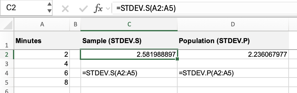
Both formulas use A2:A5. You don't need to calculate the mean in another cell first, and you shouldn't include either result cell in the input range.
Why is the sample result larger?
The four values have a mean of 5. Subtract 5 from each value, then square each difference:
| Value | Difference from 5 | Squared difference |
|---|---|---|
| 2 | -3 | 9 |
| 4 | -1 | 1 |
| 6 | 1 | 1 |
| 8 | 3 | 9 |
| Total | 20 |
Both calculations start with that total of 20. The difference is what happens next:
- STDEV.S divides by one less than the number of observations: 20 ÷ 3. The square root is approximately 2.582.
- STDEV.P divides by the number of observations: 20 ÷ 4. The square root is approximately 2.236.
Those divisors are often written as n − 1 and n, where n is the number of numeric observations. The sample calculation adjusts for estimating variation in a larger population from a limited set of observations. With the same nonidentical values, dividing by n − 1 produces the larger result. As n grows, the percentage difference between the two results becomes smaller.
The step before taking the square root is variance. If you also need that measure, see how to find variance in Excel. Standard deviation brings the result back to the original units: minutes here, rather than squared minutes.
What does the result tell you?
For these four packing times, STDEV.P describes a spread of about 2.24 minutes around a mean of 5 minutes. A smaller standard deviation means the values cluster more closely around their mean; a larger one means they're more spread out.
It doesn't mean every order takes between 5 − 2.24 and 5 + 2.24 minutes. Our values of 2 and 8 already fall outside that interval. Standard deviation alone also doesn't establish that the data follows a normal distribution.
To describe where one observation sits relative to the mean, you can use the standard deviation in a z-score calculation. Keep the same sample-or-population choice throughout that calculation.
Check what Excel includes in the range
When you supply a cell range, both functions count numeric values. That includes zero, but excludes ordinary text, numbers stored as text, logical values, and empty cells.
| Content of a referenced cell | Included? |
|---|---|
Number such as 6 | Yes |
Number 0 | Yes |
| Empty cell | No |
Text such as Missing | No |
Number stored as text, such as an entry typed as '6 | No |
Logical value TRUE or FALSE | No |
Error value such as #N/A | Causes an error result |
This matters with imported data. If A4 looks like 6 but is stored as text, STDEV.S(A2:A5) uses only the other three numbers. Check the source values before trusting a result that differs from your expected calculation. Don't replace missing observations with zero unless zero is the actual measurement.
Values typed directly into the argument list behave differently. For example:
=STDEV.S(2,4,"6",8)Here, Excel counts the quoted "6" as a number. Direct logical arguments also count: TRUE contributes 1 and FALSE contributes 0. Text that cannot become a number, or a direct error argument, causes an error. A formula with individual arguments therefore isn't always equivalent to a formula referencing cells that contain the same-looking values.
An error in the referenced range also passes through to the result: if A4 contains #N/A, both STDEV.S(A2:A5) and STDEV.P(A2:A5) return #N/A. Inspect the source error before changing functions. Replacing it with zero adds a measurement to the calculation; it doesn't repair the source data.
What about STDEV and STDEVP?
Older workbooks may use STDEV for a sample or STDEVP for a population. Microsoft retains STDEV and STDEVP for backward compatibility and points readers to STDEV.S and STDEV.P for new work.
Before you use the result, check two things: the function matches the group you mean to describe, and the range contains the numeric observations you meant to include.