To apply strikethrough in Excel for Windows, select a cell or range and press Ctrl+5. Press it again to remove the line. Microsoft's documented Mac shortcut is Shift+Command+X. You can also open Format Cells > Font and turn Strikethrough on or off.
Strikethrough keeps the cell's contents readable while drawing a line through them. It's useful for marking a finished task without deleting it. If Excel has crossed out a formula result unexpectedly, though, check the cause before changing the font: Microsoft 365 can use a similar line to flag a result that needs recalculating.
Use the Strikethrough Shortcut
Select the cell or range you want to cross out, then use the shortcut for your desktop app:
| Excel app | Apply or remove strikethrough |
|---|---|
| Windows | Ctrl+5 |
| Mac | Shift+Command+X |
These are the combinations in Microsoft's Excel keyboard shortcut reference. Its shortcut tables use a US keyboard layout.
For example, enter Send revised quote in A2. Select A2 and apply strikethrough. The words remain in the cell, with a line through them. Apply the shortcut again and the line disappears.
Select a range before applying the shortcut if you want to format several cells. To cross out only one word inside a cell, select the characters while editing instead; the partial-text steps are below.
Apply or Remove Strikethrough with Format Cells
The dialog is useful when you want to choose the setting explicitly:
- Select the cell or range.
- Press Ctrl+1 on Windows or Command+1 on Mac to open Format Cells.
- Select Font.
- Under Effects, check Strikethrough to add the line, or clear it to remove the line.
- Choose OK.
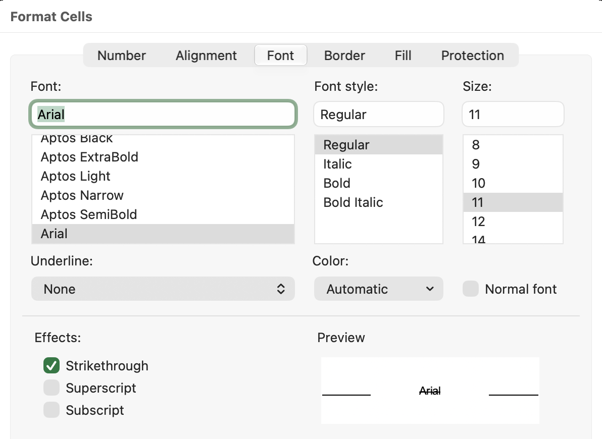
Microsoft's text-formatting instructions also describe opening the Font settings from the Home tab's dialog launcher.
If you only want to remove strikethrough, change that one setting. Clear Formats removes other formatting too, so it can undo work you meant to keep, such as number formats and fills.
Cross Out Only Part of a Cell's Text
You can mark one word without crossing out the rest of a text entry. Using Send revised quote in A2:
- Make sure A2 has no whole-cell strikethrough applied.
- Double-click A2 to edit its text.
- Highlight only revised.
- Open Format Cells, select Font, and enable Strikethrough.
- Choose OK, then press Enter or Return to finish editing.
The result should look like this: Send revised quote. The spaces and the other two words stay plain.
To remove that partial line, edit the cell again, select revised, and clear the same setting. Selecting the cell alone changes the formatting scope; selecting the characters lets you target the word.
Use this method for text entered directly in a cell. It doesn't let you format selected words within a formula's displayed result.
Mark Completed Tasks in a Small List
You can download the strikethrough example workbook to see the completed task list.
Put Task in A1 and Done? in B1, then enter these three tasks:
| Row | A: Task | B: Done? |
|---|---|---|
| 2 | Send revised quote | Done |
| 3 | Confirm delivery date | Open |
| 4 | File invoice | Done |
Select A2 and apply strikethrough. Do the same for A4, leaving A3 plain. You can still read all three tasks, and the two finished items are crossed out.
This is manual formatting. Changing B3 from Open to Done won't cross out A3 automatically; you need to apply the effect yourself. Likewise, if you reopen the quote task, change B2 to Open and remove A2's strikethrough.
Keep the status in its own column if you'll need to use it later. A line through the task name changes its appearance, but doesn't create a completion value. For a clickable state and a completion count, build a checklist with in-cell checkboxes.
If you'd prefer a visible tick beside each finished item, insert a check mark symbol. The symbol becomes cell text; strikethrough is a font effect applied to the text already there.
Why Is a Formula Result Crossed Out?
In Excel for Microsoft 365 on Windows or Mac, a crossed-out result can indicate a stale value: the inputs changed, but the formula hasn't recalculated. Microsoft documents this in Manual calculation mode and certain cases in Partial calculation mode. See its stale-value formatting guide.
Use Calculate Now on the Formulas tab to recalculate. When calculation completes, the stale-value line should disappear and the result should reflect the current inputs.
Turning off Format Stale Values only hides the indicator. It doesn't update the result. This is why treating every crossed-out number as an unwanted Font setting can miss the real problem.
The feature has exceptions, including external-data values and formulas that depend on Data Table cells. An absent strike line isn't proof that every result is current.
Remove a Line That Keeps Coming Back
Start with the affected cell and check what controls its appearance:
| What you find | What to change |
|---|---|
| Strikethrough is enabled in Format Cells > Font | Clear the setting. For a partially formatted text entry, select the affected characters first. |
| Microsoft 365 marks the formula result as stale | Recalculate the workbook rather than merely hiding the indicator. |