Your lookup key is right there in the table, but VLOOKUP returns #N/A—or brings back the wrong product. Start with three checks: use FALSE for an exact lookup, compare the stored value types, and look for extra characters. Ordinary VLOOKUP is not case-sensitive, so changing apple to APPLE won't repair a failed match.
The examples below use one product list so you can follow each problem from input to result. If you need a first walkthrough of the arguments, start with using VLOOKUP in Excel.
Download the VLOOKUP text troubleshooting workbook to follow the product-key examples, compare text and numeric inputs, and try the cleanup and wildcard formulas.
Start with a small exact-match test
Put this product list in A1:C7, with Key, Product, and Price as the headers. Enter A5 as the number 107. Enter A6 as '00107: the leading apostrophe tells Excel to store the identifier as text and isn't part of the key.
| Row | Key in column A | Product in column B | Price in column C |
|---|---|---|---|
| 2 | A-104 | Mug | 12.50 |
| 3 | A-105 | Jug | 18.00 |
| 4 | A-108 | Marker | 7.00 |
| 5 | 107 (number) | Cable | 30.00 |
| 6 | 00107 (text) | Gift box | 25.00 |
| 7 | A?108 | Sample kit | 9.00 |
Enter A-104 in F2, then put this formula in G2:
=IFERROR(VLOOKUP(F2,$A$2:$C$7,2,FALSE),"No exact key")The result should be Mug. VLOOKUP searches column A, the first column of the specified range, and returns the product from its second column. The dollar signs keep the product range fixed when you copy the formula down. To return the price, change 2 to 3:
=IFERROR(VLOOKUP(F2,$A$2:$C$7,3,FALSE),"No exact key")For A-104, that returns 12.50 when formatted to two decimal places. See the VLOOKUP reference for the full syntax.
Here, IFERROR gives unsuccessful examples a readable label. It does not fix the lookup, and it catches errors other than missing keys. If this label appears unexpectedly in your own report, inspect the underlying formula and error before assuming the key is absent. The Excel formula errors guide explains what those error values mean and where to check next.
Keep FALSE as the fourth argument
FALSE selects exact-match mode. TRUE, or leaving the fourth argument out, selects approximate matching and requires the first column to be sorted. Approximate matching is useful for bands and thresholds; it isn't a way to find part of a product code. VLOOKUP's fourth argument explained walks through that choice.
There is one catch: exact-match mode still interprets wildcard characters in a text lookup value. We'll check that separately below. Microsoft's VLOOKUP documentation describes both match modes and the wildcard rules.
Check the value type before changing the format
A numeric 107 and the text string 107 can look identical. Changing the cell's number format doesn't, by itself, convert an existing text value into a number.
Use these inputs in F2:F11. Copy the product formula from G2 down to G11; the results column below shows what to expect before applying any repairs.
| Input cell | What to enter | Expected product result |
|---|---|---|
| F2 | A-104 | Mug |
| F3 | a-104 | Mug |
| F4 | A-104, with one space at each end | No exact key |
| F5 | A-10? | Mug |
| F6 | A-10* | Mug |
| F7 | A?108 | Marker |
| F8 | 107 as a number | Cable |
| F9 | '107 to store text | No exact key |
| F10 | '00107 to store text | Gift box |
| F11 | The formula shown below | No exact key |
In F11, enter a leading ordinary space and a trailing nonbreaking space with this formula:
=" "&"A-104"&UNICHAR(160)UNICHAR selects a character by its Unicode number, as Microsoft's UNICHAR documentation explains. Here, 160 selects the nonbreaking space U+00A0. CHAR uses your computer's character set instead; Microsoft's CHAR documentation distinguishes Windows and Macintosh mappings. Use UNICHAR(160) when you need this specific Unicode space, rather than assuming CHAR(160) produces it on every platform.

Now check the stored types in spare cells. TYPE returns 1 for a number and 2 for text:
=TYPE(A5)That should return 1. Change the reference to A6 and it should return 2. Likewise, =TYPE(F9) should return 2. For a direct numeric check, use ISNUMBER:
=ISNUMBER(F8)The result should be TRUE; the same check on F9 should be FALSE. Cell alignment can be a hint, but these checks tell you what Excel actually stores.
Convert numeric text only when it represents a numeric key
F9 contains text 107, while the Cable key in A5 is numeric. In this case, VALUE makes the types agree:
=IFERROR(VLOOKUP(VALUE(F9),$A$2:$C$7,2,FALSE),"No exact key")The result should now be Cable. This repair is appropriate because F9 is supposed to identify the numeric key 107. For imported amounts with decimal or thousands separators, see converting text to numbers in Excel.
Don't apply it to every identifier. Text 00107 belongs to Gift box in this list. Converting that value to a number removes its leading zeroes and changes the lookup to 107, which belongs to Cable. Keep significant leading zeroes as text on both sides of the lookup. If Excel already removed them during import, changing the display format can't recover the original identifier reliably.
Count extra characters, then clean both sides
F4 looks much like F2, but the spaces count. Use LEN to compare their lengths:
=LEN(F4)The padded value has 7 characters; A-104 has 5. =LEN(F11) also returns 7, even though its final character is a nonbreaking space. A length difference flags extra characters; it doesn't identify them, and equal lengths don't prove two keys are identical.
Choose the cleanup for the characters you have:
- TRIM removes ordinary ASCII spaces at the ends and reduces repeated ordinary spaces between words to one. It doesn't remove every kind of whitespace.
- CLEAN removes ASCII control characters 0–31, such as tabs and line breaks. It doesn't remove every invisible Unicode character.
- SUBSTITUTE can replace a specific unwanted character. In this example,
UNICHAR(160)supplies the nonbreaking space to replace with an ordinary space.
These limits are documented in Microsoft's guide to cleaning data. If a different Unicode character remains, identify that character and target it; stacking TRIM and CLEAN isn't a universal repair.
Build a helper lookup range
Cleaning only the input won't help if the source keys contain unwanted characters too. Use D:E as a helper range, leaving the originals available for comparison.
Enter Clean key in D1 and Product in E1. In D2, enter:
=TRIM(SUBSTITUTE(CLEAN(A2),UNICHAR(160)," "))Copy D2 down through D4, then copy it to D6:D7. These are the text-key rows. In D5, preserve the numeric Cable key with:
=A5Enter =B2 in E2 and copy down to E7. Now normalize the padded lookup input and search the helper range:
=IFERROR(VLOOKUP(TRIM(SUBSTITUTE(CLEAN(F4),UNICHAR(160)," ")),$D$2:$E$7,2,FALSE),"No exact key")The result should be Mug. Replace F4 with F11 in that formula to check the nonbreaking-space input; it should also return Mug. The cleaned keys have five characters.
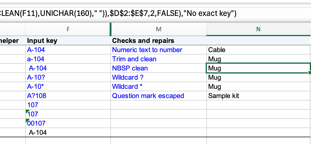
Only remove characters that are unwanted. TRIM changes repeated internal spaces, and CLEAN deletes control characters rather than replacing them with separators. Those changes could merge two meaningful keys in another dataset. Compare the helper values with the originals before using them in a report.
Letter case isn't the mismatch
F2 contains A-104; F3 contains a-104. Both lookups should return Mug because ordinary VLOOKUP ignores differences between uppercase and lowercase letters.
You don't need to convert the keys to uppercase or lowercase to make those two values match. If your business rules treat differently cased identifiers as separate items, ordinary VLOOKUP doesn't distinguish them; changing the case would lose that distinction as well.
Separate wildcard matches from approximate matches
With FALSE, text lookup values can still contain patterns:
| Character | Meaning in the lookup value | Example |
|---|---|---|
? | Any one character | A-10? |
* | Any sequence of characters | A-10* |
~ before a wildcard | Match the literal symbol | A~?108 |
_ | An ordinary underscore | A_104 |
An underscore is not a VLOOKUP wildcard.
F5 contains A-10?. This formula should return Mug, because A-104 is the first matching key:
=IFERROR(VLOOKUP(F5,$A$2:$C$7,2,FALSE),"No exact key")Using F6, which contains A-10*, also returns Mug. Both patterns match several keys in this product list; VLOOKUP returns the first matching row, not a list of matches.
Escape a question mark that belongs to the key
F7 contains A?108. You might expect Sample kit, but this formula should return Marker:
=IFERROR(VLOOKUP(F7,$A$2:$C$7,2,FALSE),"No exact key")The question mark matches the hyphen in A-108, and that row comes before A?108. To search for the literal question mark, put a tilde before it:
=IFERROR(VLOOKUP("A~?108",$A$2:$C$7,2,FALSE),"No exact key")Now the result should be Sample kit. Use ~* for a literal asterisk and ~~ for a literal tilde. Keeping FALSE is still correct; escaping the character changes how Excel reads the lookup text.
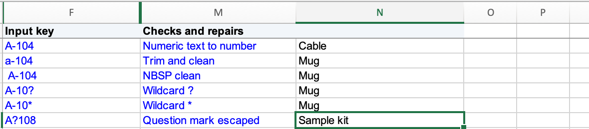
Duplicate source keys create a similar first-row problem even without wildcards. If two rows have the same key, VLOOKUP doesn't decide which product you intended. Check duplicates before trusting a plausible result.
If the lookup still fails
Check these in order:
- Range and return column: The key must be in the first column of the lookup range. For A2:C7, product is column
2and price is column3. - Match mode: Use
FALSEfor these product keys. A missing fourth argument selects approximate matching. - Stored type: Compare TYPE or ISNUMBER results. Convert only when doing so preserves the key's meaning.
- Actual characters: Compare lengths and inspect spaces, punctuation, and imported characters on both sides.
- Patterns and duplicates: Escape literal wildcard symbols and check whether an earlier row also matches.
- Missing key: Confirm the requested identifier really exists within the selected range. A clean, correctly typed value can still be absent.
If the key column needs to sit to the right of the result column, using INDEX and MATCH together gives you a more flexible layout. It still needs consistent keys.