To make a waterfall chart in Excel, select a starting balance and the positive and negative changes, then insert a Waterfall chart. Select each balance or subtotal column individually and choose Set as Total so it starts at zero. That last step matters: Excel needs to know which values are balances and which are changes.
Suppose you start with 100 in cash, receive money from customers, and make several payments. We'll build a chart that explains why you finish with 95, including a subtotal before operating payments.
Arrange the source data: changes and balances
A waterfall chart, also called a bridge chart, shows how individual increases and decreases move a starting amount to an ending amount. Use it when the question is “What caused the change?” If you already have a balance for every month and want to show its trend, a line graph in Excel may fit that task better.
For this example, create a worksheet named Bridge. Enter Stage in A1 and Amount in B1, then fill rows 2–8 as shown. Keep all amounts in the same unit.
| Row | Column A: Stage | Column B: Amount or formula | Expected value |
|---|---|---|---|
| 2 | Opening cash | 100 | 100 |
| 3 | Customer receipts | 60 | 60 |
| 4 | Customer refunds | -10 | -10 |
| 5 | Supplier payments | -25 | -25 |
| 6 | Cash before operating payments | =B2+B3+B4+B5 | 125 |
| 7 | Operating payments | -30 | -30 |
| 8 | Closing cash | =B6+B7 | 95 |
Enter this formula in B6:
=B2+B3+B4+B5It returns 125: the opening 100 plus receipts of 60, less refunds of 10 and supplier payments of 25.
In B8, enter:
=B6+B7It returns 95. B7 already contains a negative number, so adding B7 subtracts the operating payment. Don't subtract B7 again; that would turn the payment into an increase.
Rows 3, 4, 5, and 7 are changes. Rows 2, 6, and 8 are balances. For example, B3 contains the receipt of 60, not the resulting cash balance of 160. Excel uses the changes to position the floating columns.
Check the ending balance before charting
Leave row 9 blank. In A10, enter Check excluding subtotal. In B10, enter:
=B2+B3+B4+B5+B7This independently adds the opening balance and each cash movement, leaving out the subtotal in B6 and closing balance in B8. B10 and B8 should both show 95.
100 + 60 - 10 - 25 - 30 = 95Don't add every value in B2:B8 to calculate closing cash. That would give 315 because it includes the subtotal of 125 and the closing balance of 95 on top of the opening cash and movements. Those summary rows repeat amounts already accounted for.
You can follow along in the waterfall chart practice workbook. The Bridge sheet includes the cash movements, subtotal and closing-balance formulas, an independent check, and the completed chart.
Insert the native Waterfall chart
Select A2:B8. Include both the stage labels and amounts, but leave the check in row 10 outside the chart.
In desktop Excel, open Insert, choose the Waterfall chart menu, and select Waterfall. On Windows, the menu is labeled Insert Waterfall…; on Mac, look for the Waterfall icon. Microsoft's waterfall chart instructions cover both platforms.
The chart should contain seven columns in worksheet order. Before you judge the result, identify the three balance columns as totals.
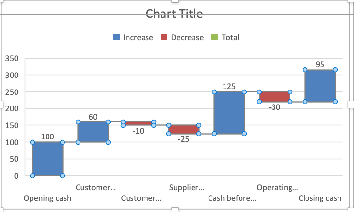
Set the opening balance, subtotal, and closing balance as totals
Work with one chart column at a time:
- Select the Opening cash column. If the whole series is selected, click that column again to isolate the point.
- Right-click the selected point and choose Set as Total. Alternatively, open Format Data Point and select Set as total.
- Repeat for Cash before operating payments, the subtotal from B6.
- Repeat for Closing cash, the balance from B8.
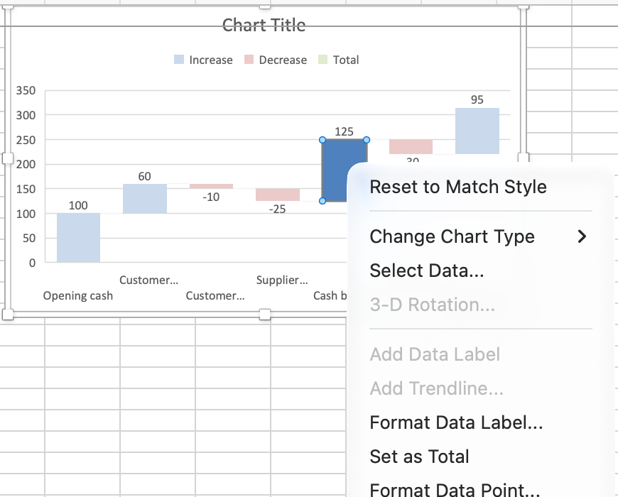
After you apply Set as Total to all three balance columns, they should extend from zero to 100, 125, and 95, respectively. Leave Customer receipts, Customer refunds, Supplier payments, and Operating payments as changes.
If the menu says Format Data Series, you've selected the whole series. Select the individual column again to reach Format Data Point. The distinction is easy to miss when several columns have selection handles.
Setting a point as a total changes how the chart treats it. It doesn't calculate a subtotal for you or repair the worksheet formula. B6 must already contain 125, and B8 must already contain 95.
Once the totals are set, replace Chart Title with a descriptive title such as Cash bridge.
Read the finished chart
Follow the chart from left to right and compare it with this sequence:
| Stage | Expected position |
|---|---|
| Opening cash | Total from 0 to 100 |
| Customer receipts | Increase from 100 to 160 |
| Customer refunds | Decrease from 160 to 150 |
| Supplier payments | Decrease from 150 to 125 |
| Cash before operating payments | Subtotal from 0 to 125 |
| Operating payments | Decrease from 125 to 95 |
| Closing cash | Total from 0 to 95 |
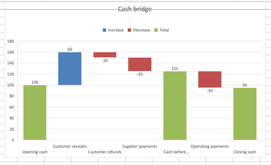
Keep connector lines visible while checking the flow. In Format Data Series, use Show connector lines to turn them on or off. They help you follow the running balance between changes.
Check the labels as well as the column heights. The Customer receipts amount is 60, even though its upper edge reaches 160. One number is the movement; the other is the cash balance after that movement.
Fix floating totals and wrong results
The subtotal or closing balance floats
Select that point and apply Set as Total. A floating summary column is being treated as another change. For example, the 125 in B6 is cash on hand at that stage, not an additional receipt of 125.
A payment increases the balance
Check the sign in the source cell. B4, B5, and B7 must contain -10, -25, and -30. A label such as “Supplier payments” doesn't tell Excel to subtract the value.
The worksheet total is wrong
Compare B8 with the independent check in B10. Check for a missing movement, a reversed sign, or a subtotal included twice. Changing a chart setting won't correct the source calculation.
The worksheet is right, but the chart is wrong
Check that the chart uses A2:B8 and that only the points from rows 2, 6, and 8 are marked as totals. A change marked as a total starts from zero and breaks the intended sequence. Clear Set as total for that point.
Finally, check that your data describes one consistent measure. This example follows cash throughout; revenue or profit figures can't replace cash receipts and payments without changing what the chart means. If your question is about the relationship between two measurements, such as order size and delivery cost, use a scatter plot for that separate task.