If you need to calculate hours between two dates and times in Excel, the simplest formula is to subtract the start date and time from the end date and time. From there, you can either show the result as elapsed time or convert it to decimal hours.
Quick Answer
If A2 contains the start date and time and B2 contains the end date and time, use:
=B2-A2
To return decimal hours instead of a time value, use:
=(B2-A2)*24
If you want to display the result as total elapsed hours and minutes, format the result cell as:
[h]:mm
Example: Hours Between Two Date-Time Values
Suppose:
A2=1/20/2022 6:00 AMB2=1/21/2022 2:00 PM
This formula:
=B2-A2
returns 1 day and 8 hours. If you format the result as [h]:mm, Excel shows 32:00.
If you want the answer as a number, use:
=(B2-A2)*24
and Excel returns 32.
Calculate Hours When Date and Time Are in Separate Cells
Many worksheets store dates and times in separate columns. In that case, add the date and time together before subtracting.
Assume:
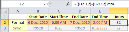
A2= Start dateB2= Start timeC2= End dateD2= End time
Use:
=(C2+D2)-(A2+B2)
To return decimal hours:
=((C2+D2)-(A2+B2))*24
This is often easier to audit than typing a full timestamp into one cell.
Show Elapsed Hours Above 24
One of the most common mistakes is using a normal time format for a duration.
If the result of =B2-A2 is formatted as a standard time, Excel may show only the clock portion of the answer. That means a 32-hour duration can look like 8:00.
To show total elapsed hours, use a custom format:
[h]:mm
If you need seconds, use:
[h]:mm:ss
For a deeper explanation of elapsed time formatting, see Let Excel Convert Hours Between Two Dates and Times.
Return Decimal Hours, Minutes, or Seconds
If you need a numeric result for payroll, billing, or reporting, multiply the time difference by the right conversion factor.
Decimal hours:
=(B2-A2)*24
Minutes:
=(B2-A2)*1440
Seconds:
=(B2-A2)*86400
If you later need to turn decimal hours back into a time display, see How to Convert Decimal Hours to Time in Excel.
Calculate Time Across Midnight
If your cells contain full date-time values, a basic subtraction already handles overnight spans:
=B2-A2
For example, if A2 is 3/15/2026 10:00 PM and B2 is 3/16/2026 6:00 AM, the result is 8 hours.
If you are working with times only and the shift crosses midnight, use:
=MOD(B2-A2,1)
That prevents a negative time result when the end time belongs to the next day.
For related techniques, see How to Extract Time from DateTime Values in Excel and Extract Time with the MOD Function in Excel.
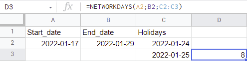
Exclude Weekends and Holidays
If you want working hours rather than raw elapsed hours, NETWORKDAYS or NETWORKDAYS.INTL is the better starting point.
For example, to count working days between two dates:
=NETWORKDAYS(A2,B2,HolidayList)
You can then multiply that result by the number of hours in a standard workday.
If your first and last days are partial days, the setup becomes more advanced because you need to account for:
- workday start time
- workday end time
- weekend pattern
- optional holiday list
That is a different problem from simple elapsed time, so it is best handled with a dedicated working-hours formula.
Why the Formula Works
Excel stores dates as whole numbers and times as fractions of a day. That is why ordinary subtraction works for date-time calculations.
In Excel:
1= one full day0.5= 12 hours0.25= 6 hours
So when you subtract one timestamp from another, Excel returns the elapsed fraction of a day. Multiplying by 24 converts that fraction into hours.
If you need a live calculation based on the current time, the NOW function can help:
=(NOW()-A2)*24
Common Problems
The result shows 8:00 instead of 32:00
Use the custom format [h]:mm so Excel shows accumulated hours instead of wrapping after 24.
I want a number, not a time
Multiply by 24:
=(B2-A2)*24
My result is negative
Make sure the end date and time are later than the start date and time. If you only have times and the period crosses midnight, use =MOD(B2-A2,1).
Excel shows hash marks instead of a result
This usually means the cell is not wide enough or Excel is trying to display a negative time value in a time format.
Should I use DATEDIF?
Usually no. DATEDIF is best for date-only differences in years, months, or days. For hours between timestamps, subtraction is simpler. If you need date-only intervals, see the DATEDIF function in Excel.
Formula Summary
Use =B2-A2 for elapsed time.
Use =(B2-A2)*24 for decimal hours.
Use =((C2+D2)-(A2+B2))*24 when dates and times are stored separately.
Use =MOD(B2-A2,1) when you only have times and the shift crosses midnight.
Once you understand that Excel measures time as a fraction of a day, calculating hours between two dates and times becomes straightforward.
For more date and time tutorials, browse the Date & Time section or read 4 Methods to Insert a Timestamp in Excel Cell.