Category Archives: Time and Date

How To Calculate Hours Between Two Dates in Excel

Recently I was asked how to subtract time in Excel (time difference) or how to calculate the number of hours between two points in time on different days. Since this was in a reader comment, I gave a brief answer that requires a fuller account here.

Dates and Times are all part of the master plan in Excel. Once you “get” the fundamentals, the rest is just icing on the cake.

A Date value in Excel looks like this: 40519
A Time value in Excel looks like this: 0.58333

Cell formatting changes how you see these numbers.

The Date: 7 Dec, 2010
The Time: 2:00 PM

How to Calculate Time Between Dates in Excel or the Duration Between Two Dates

If you want to calculate time between dates in Excel or the duration between two dates, you need to understand what they mean first. When you type a Date into Excel, you may never see the underlying number, like 40519, but it’s there nonetheless. This is a date serial number and it makes Date calculations easy.

You might ask, “Why is this such a weird-looking number?”. Well, the Excel folks started a numbering system with Dates. In Excel for Windows they gave 1 Jan, 1900 the serial date number of 1, then continued numbering until this day and beyond. So serial number 40519 represents 7 Dec, 2010.

In Excel for Mac they started numbering Dates beginning with 2 Jan, 1904. (don’t ask) So the serial date 40519 represents 8 Dec, 2014 (Actually it’s known as the 1904 date system. To be clear, Macs can change Excel settings to use the 1900 date system).

How to Subtract Time in Excel (Time Difference)

When you type 2:00 PM into a cell in Excel the underlying value is a fraction, but Excel interprets this as a time serial number and formats the cell accordingly.

Try typing 0.25 into a blank cell, then change the cell formatting to a TIME format, and you’ll get something like 6:00 AM.

As an aside, you can calculate this fraction for any time value during the day by taking the total number of seconds that have passed from midnight until your time value and dividing by 86,400 seconds in a day.

Dates and Times Together

In Excel the unit of time is “the Day,” a key fact to know. You’ll notice that Dates are integers, and Time is a fractional number. You can add the two together to get a Date/Time format.

So adding a Date serial number, like 40518, to a Time serial number, like 0.25, gives us 40518.25. Formatting the cell holding this value using “d mmm, yyyy h:mm AM/PM” will show 6 Dec, 2010 6:00 AM.

You can also enter something like 7 Dec, 2010 2:00 PM into a cell and Excel will recognize this as a Date/Time format. However, if you change the cell formatting to General, the underlying number is 40519.05833.

So hopefully by now you can see that subtracting two Date/Time formatted numbers can be done mathematically. Subtracting 6 Dec, 2010 6:00 AM from 7 Dec, 2010 2:00 PM is done by Excel “underneath the hood” as 40519.05833 – 40518.25 and the result is 1.3333.

Calculating Hours Between Two Dates in Excel

If we recall that the unit of time is “the Day,” this value represents 1-1/3 days of time. Since there are 24 hours in a day, converting to hours is a simple multiplication 24 * 1.3333 = or 32 hours. (24 * 4/3 to be more precise)

Time Between Two Times / Dates

Finding the number of hours or the time between two times/dates is simple, just subtract the start date/time from the end date/time and multiply the result by 24 hours.

If you want to enter the dates and times separately (which is loads easier than typing in a date/time in one cell) then add the date/times together.

Hours = ((End_Date+End_Time)-(Start_Date+Start_Time))*24

Here’s a look at a typical worksheet designed to calculate the hours between two dates.

As you can see, the formula for Hours, in cell F2, shows in the formula bar. And row 3 contains General formatting so you can view the date/time serial numbers for row 2.

Change the formatting for cells B2:E2 to match what you normally use for Date and Time data entry.

The NETWORKDAYS Function

People also asked how to calculate the time between days but without taking into account weekends or specified holidays. The NETWORKDAYS function will help you to calculate the time period by excluding weekdays and specified holidays.

The formula looks like this: =NETWORKDAYS(start_date, end_date, [holidays])

Like in the previous case the start_date and end_date are required arguments, yet the argument [holidays] is optional. You can use this argument to specify which days should be excluded.

This time I used two random dates which contained two weekends and I added two desired dates under the holidays argument just to show you how it works.

If you need to add some weekends you will have to add one more argument (weekends) and use =NETWORKDAYS.INTL(start_date, end_date, [weekend], [holidays])

After you calculated the days by using the NETWORKDAYS formula, to calculate the hours you can simply multiply the given number with the number of hours you need for as long as they stay the same. Also, do not work harder by looking for complicated formulas to calculate simple things.

What else you should know:

If the start date is later than the end date the formula will generate a negative number.
The NETWORKDAYS formula will also include the start and the ending dates in the calculations, due to this if you have the same date the value returned will be 1.

If you want to find more formulas regarding the date and time feel free to check the following list of functions.

I hope this article helps you to better understand how to calculate hours between two dates in Excel. You can exercise what you learned today by calculating the time left until your next birthday, to do this you can also use the =Today function or the =Now function.

If you found this article helpful, please feel free to check our other articles about tips and tricks in Excel. We also have a dedicated section for details and formulas about dates and times in Excel.

Extracting Integers and Fractions in Microsoft Excel

Sometimes you need to extract the integer portion of a number. Sometimes the fractional part. Sometimes both. Excel makes it easy to get the integer and somewhat harder to get the fraction. If you just want the answer, skip to the technical details.

The Integer Part: Excel INT Function

What could be easier than the Excel INT function? I mean INT almost screams INTEGER. So the name is intuitive. You almost “know” what it’s going to do, even if you haven’t used it before.

With only one argument, it’s execution is even simpler. Just feed it a number and out pops the integer portion.

Below you can see I have the number 14.125 in cell D1 and the formula =INT(D1) returns the integer 14 in cell E1.

Date/Time Tip: A practical application for the INT function is to extract the date value from a date/time number. An example is a date/time value like 2/14/2013 9:04 AM in cell A2 and you only want the date. Using the formula =INT(A2) will strip out the time and leave the date 2/14/2013.

The Fractional Part

Here is where I would like some simplification. I mean, if we have the INT function for extracting an integer, you would think that there would be a FRAC function, or a simple name like that, to extract the fractional part.

If there was a FRAC function, you could also imagine that it would have only one argument. Just feed it a number and out pops the fraction. Simple. Elegant. Intuitive. No thought required. But, I digress.

To extract the fractional part of a number we can use the MOD function, which has not one, but two arguments. The reason it has two arguments is because it does more than extracting the fractional part. Forget about that.

Here is what you need to know about the MOD function and how to extract the fractional part of a number. The second argument of the MOD function is 1. Remember that. To reiterate, 1 is the second argument.

The first argument of the MOD function is the number. Shown below, you can see the number 14.125 in cell D1. The formula =MOD(D1,1) returns the fractional part 0.125 in cell E1.

Date/Time Tip: A handy way to extract a time value from a date/time number is to use the MOD function. Per our previous example, the date/time number 2/14/2013 9:04 AM in cell A2, the formula =MOD(A2,1) will return 9:04 AM.

Technical Details

Assume you have a number in cell A1.

To extract the integer value, use the formula:
=INT(A1)

To extract the fractional value, use the formula:
=MOD(A1,1)

Extract Time with the MOD Function in Excel

I had a reader comment on my last post about how to extract time from a date-time number using the MOD function. Simple really.

The syntax is MOD(number,divisor). The MOD function returns the remainder after number is divided by divisor. A simple example is MOD(5,2), which equals one (1). It works like this: five (5) divided by two (2) equals two (2), with one (1) left over.

All numbers are evenly divisible by one (1) so the MOD function returns any fractional part when the second argument is one (1).

In the screen shot below, cell C2 has the Date-Time number: 10/8/12 6:28 PM. It has an underlying serial number: 41990.7698, which you can see in cell C3 with General formatting.

Using the formula =MOD(C2,1) you can see the result in cells D2 and D3, with different cell formatting. Extracting the Time value from a Date-Time value is simple with the MOD function.

Extract Time from a Date-Time Number in Excel

I have a worksheet that tracks start and stop times for different events throughout the day, all during the week. Sometimes I have to pull out the Time of Day, irrespective of the Date, with the TIME function.

The TIME function has three arguments: Hour, Minute, Second. I could use =TIME(11,30,0) in a cell to get 11:30 AM, but I want to convert a Date-Time number so let’s look at an example.

In cell C2 I have the Date-Time value 10/8/12 6:28:30 PM.

In cell B2 I enter the formula =TIME(HOUR(C2),MINUTE(C2), SECOND(C2)) to pull out the time value. Notice that the HOUR, MINUTE, and SECOND functions are used to extract values for the Hour, Minute, and Second arguments. The TIME Function puts these into a nicely formatted time value of 6:28 PM.

Now the Time values can be used independently of the Date.

Note: You don’t see the 30 seconds in cell B2 because of the default cell formatting for Time in my spreadsheet.

A Shortcut Formula [UPDATE]

I had a reader comment about an easier formula so I will include it in this post. Thanks JMarc.

A Date-Time serial number, with General formatting, shows up as an Integer.Fraction. You don’t normally see this on your spreadsheet as Excel will automatically format Date-Time numbers as, well, Date-Time numbers.

The screen shot below shows the Date-Time number and its serial number equivalent with General formatting. Both underlying numbers are identical, the cell formatting is the only difference.

The INT function returns the integer portion of a number. If we use the Date-Time number and subtract the integer portion, that leaves us with the fractional portion, which is the Time. The formula =C2-INT(C2) will return the number 0.769795602.

Reformatting the cell to a Time format will allow the fraction to show as a Time value.

Changing the cell formatting gives us the time value 6:28 PM.

Extract a Date from a Date-Time Number in Excel

I recently saw a spreadsheet with the following function =LEFT(A2,8) where cell A2 was equal to 08/06/12 12:23 PM. The user was trying to extract the Date from the Date-Time value. The problem for me was that the LEFT function returns a “text” value. Excel is good at recognizing text values that look like dates, as Dates, but why not use a formula that returns a numeric value?

My reflex was to enter the following formula =DATE(YEAR(A2),MONTH(A2),DAY(A2)) and get a proper Date value. You can tell the difference because, with no cell formatting, a Text value is left-justified in the cell, and a Date value is right-justified in the cell, meaning that it’s a number.

I got to thinking later that there’s a simpler formula to extract the Date from a Date-Time value, which is =INT(A2). After you enter this formula, the cell formatting needs to be changed to a Date format.

Why Does the INT Function Extract a Date?

All Dates, Times, and Date-Times are know as serial numbers in Excel. You don’t normally see the underlying serial number. A Date-Time value like 9/14/2012 8:43 AM looks like that in the cell AND in the formula bar.

Date Time shown in Cell and Formula Bar

Only when you change the cell formatting to General do you see the Date-Time serial number. The integer portion is the date serial number and the fractional part is the time serial number.

Serial Date Time

This is why the INT function will work to extract a Date from a Date-Time value. The integer value is a date serial number. The trick is to change the cell formatting to a Date format so that Excel will show you the Date.

Format Cells Date

Pay Periods and Funky PivotTable Controls

I like to use a PivotTable to figure out simple problems in Excel. So for this post I’m going to use Excel 2011 (Mac), where PivotTable controls look funky when compared to their Windows counterpart.

Since I get paid every two weeks, certain months in a year will contain three pay periods. Planning future vacations during these months isn’t a bad idea, so I’m going to look at pay periods for the next three years.

Add a Column of Dates

I’ll enter the first pay period, then create a formula that adds 14 days and copy it down to get my date range.

Since a PivotTable will “see” the underlying serial date, I’ll need to add another column for Month and give it a “Month-Year” format so the PivotTable will group similar Months together. For this I’ll use the TEXT formula. The “Pay Period” Date is used for the first value argument, and then “mmm-yy” for the format_text argument.

So the formula in cell B3 =TEXT(A3,”mmm-yy”)

As you can see in the screen shot, the months Dec-11 and Jun-12 have three pay periods. A PivotTable will quickly summarize more than one year and show the number of times a pay period happens each month.

Add a PivotTable

The steps to create a PivotTable in Excel 2011 are as such.

Select a cell inside the data range
Click the Data tab on the Ribbon
Click the PivotTable drop-down arrow and select Create Manual PivotTable…

On the PivotTable dialog box, click OK

You’ll get a new worksheet that shows an empty PivotTable Layout. There’s an introductory PivotTable popup box that has a link to Learn more about PivotTables, which brings up the Help system topic About PivotTables. Click the x to dismiss this help box.

The PivotTable Builder box is also shown. This object looks quite a bit different from the traditional Windows counterpart. My first reaction was that it looks funky. Nevertheless, it’s the functionality that counts.

Arrange the PivotTable Layout

Click and drag Month from the Field name area to the Row Labels area. Then click Month again and drag it to the Values area. (Yes that’s right, you’re dragging Month twice.)

In the Values area you should see Count of… and to see the rest, just click the i to bring up the field name list.

Sort the PivotTable

Click inside the Data area (like cell B5) of the PivotTable and then select Descending from the Sort icon drop-down list on the Toolbar.

The top of the list shows months with 3 pay periods. Just what I was looking for.

You’ll notice the descending sort doesn’t leave the Row Labels in ascending order. (Nov-12 doesn’t follow Jun-12, etc.)

A Better Formula

You can change the Month formula to =TEXT(A2,”yyyy-mm”) and the Row Labels will show up in year-month format in ascending order.

While this took some time to explain, the reality is when I do this it takes about two minutes. And the bulk of the time is generating the dates and adding the formula.

International Short Date Formatting for the TEXT Function

I have an Excel workbook that is used in two different regions where the date format is entirely different, the US and the UK. At the top of a report worksheet I use a TEXT function to inform the user of the date range.

Here’s what a US user sees:

From: 6/6/2011 to 6/10/2011

Here is the formula:

=”From: ” & TEXT(MIN(ExtractData!A:A),”m/d/yyyy”) & ” to ” & TEXT(MAX(ExtractData!A:A),”m/d/yyyy”)

The Min and Max dates are in column A on a worksheet named ExtractData.

The problem is trying to automatically change the date format in the second argument of the TEXT Function – “m/d/yyyy” – which is a string argument. We can use VBA to accomplish this, but first a refresher on the TEXT function syntax.

The Solution

The Application.International Property solves this problem with the xlMDY argument, which is TRUE if the date order is month-day-year, and FALSE if the date order is day-month-year. This property is put into the Workbook_Open event and modifies a defined name constant that’s used for the second argument of the TEXT function.

Here’s how it’s done.

Create a Defined Name Constant for the Date Format

I created a Defined Name Constant to store a Short Date format, and gave it the name sd_format.

In Excel 2007 and 2010, choose Formulas > Define Name to bring up the New Name dialog box where you type in sd_format in the Name box, and type =”m/d/yyyy” in the Refers to box. Remember the equals sign.

In Excel 2003, 2008, and 2011 choose Insert > Name > Define to bring up the Define Name dialog box. Type sd_format in the Names in workbook box, then type =”m/d/yyyy” in the Refers to box. Be sure to use the equals sign.

Substitute the Named Constant in the TEXT Function

The sd_format defined name can now be substituted for “m/d/yyy” in the second argument of the TEXT function. Here’s the new formula:

=”From: ” & TEXT(MIN(ExtractData!A:A),sd_format) & ” to ” & TEXT(MAX(ExtractData!A:A),sd_format)

Since sd_format is already a text string, enclosed quotes are not needed.

Create a Workbook Open Routine

In the VBA Editor, I created a Workbook_Open subroutine, which looks at the computers international setting for the US, and if TRUE changes the sd_format value to “m/d/yyy”, and otherwise changes it to “d/m/yyyy” for the UK short date format.
Private Sub Workbook_Open() '''''''''''''''''''''''''''''''''''''''''''''''''''''''''''''''''' ' This routing updates the regional date setting format for the ' defined name sd_format. ''''''''''''''''''''''''''''''''''''''''''''''''''''''''''''''' If Application.International(xlMDY) = True Then ThisWorkbook.Names("sd_format").Value = "m/d/yyyy" Else ThisWorkbook.Names("sd_format").Value = "d/m/yyyy" End If End Sub

How it All Works

Each time the workbook is opened the Workbook_Open routine executes the IF-THEN-ELSE statement, which simply looks to see if the computers region setting is month-day-year, then sets the defined name sd_format to “m/d/yyyy” which is a US format. If the computer’s region setting for the long date format is NOT month-day-year (and presumably day-month-year) then sd_format is set to “d/m/yyyy” for the UK.

Every TEXT function using sd_format for the second argument will then have the proper short date format for that computer.

Note: Obviously if the region settings are changed on the computer while the file is open the file will have to be closed and reopened, but this would most likely be a rare occurrence.

Regional Date Formats in Excel

I recently returned from two weeks in Ireland where I installed a couple of Excel reporting systems and came across the dreaded regional date settings. My computer is set for the US region, whereas the client’s computers were set for the UK region. When I mention regional settings on my computer, I’m talking about Windows and not Excel.

Trying to get Excel to automatically switch date formats between computers using different region settings was something I experienced a few years ago while working in England. Back then I made the mistake of ustng Excel to change the formatting for my dates. Not the way to go.

Regional Date Formats

The US Short Date format is represented in the form “m/d/yyyy” which means dates are shown in a “Months/Days/Years” format. Contrast that with Ireland, the UK, and most everywhere else, where the date format is “dd/mm/yyyy” and takes the form Days/Months/Years.

Using the Default Short Date Format in Excel

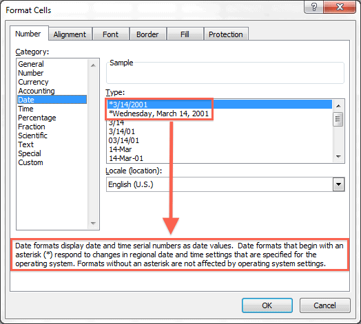
Since I live in the US my computer’s regional settings are set for the US. When formatting dates in Excel for files that may be used internationally, it’s wise to use date formats that begin with an asterisk (*) per the Format Cells Dialog box.

Any date formatted in this manner will display correctly in another region. I can view the date June 13, 2011 in my spreadsheet as 6/13/2011 and send it to a person using a UK regional setting on their computer and the date will automatically display as 13/6/2011.

Nice and neat. We’re all speaking the same language here.

How Not to Change a Date Format for a Different Locale (Region)

Let’s say you are in the US and are designing a spreadsheet that will be used in the UK. You want to see “what they see” and decide to change the cell formatting in a column that contains dates. You select the range, open the Format Cells dialog box (Ctrl+1) then select English (U.K.) from the Locale (Location) drop-down list, and click OK.

Bad move.

First of all, look at the picture above and notice there are no date formats that have a leading asterisk (*) which means that no date format will survive a change to a different region. You are stuck with this format in every region, whether it’s relevant or not.

How to Change Region Settings in Windows

The proper way to “see” a different region’s date format is to change your computer’s Region setting. Click the Windows Start button and select Control Panel. Find and click the link for Clock, Language, and Region.

Next click the link for Change the date, time, or number format.

On the Region and Language dialog box click the Formats tab.

In the Format drop-down box select the Region of your choice. In my case that’s English (United Kingdom).

In the screen shot above you can see the Short Date format is dd/MM/yyyy. Click OK to set your computer’s region.

Now open Excel and all dates previously formatted with the default Short Date format for the US (*3/14/2001) will show up in the Short Date format for the UK.

To check this fact, select a cell with dates, then bring up the Format Cells dialog box (Ctrl+1) to see that the Short Date format in Excel has automatically changed to *14/3/2001.

This is how you change the date formats for different regions.

Customize the Region Date Format in Windows

I don’t like having two digits showing for the day and month in the Short Date format. To me 4 July, 2011 should be represented as 4/7/2011 and not as 04/07/2011. However that’s what you get when you select the English (United Kingdom) region setting.

I used a custom format for the UK region short date setting to rid my spreadsheet of the unnecessary zeros. To do this you bring up the Region and Language dialog box, as we did previously, and click Additional Settings… then select the Date tab.

Type d/M/yyy in the Short Date box and click OK.

Now all months and days with single digits show up without a leading zero in Excel when using the short date format.

Quickly Adjust 1904 Dates for the 1900 Date System in Excel

An associate of mine “helped” me out once by putting a worksheet together for data entry. After the worksheet had several days of user input, I found out the workbook was created on a Mac with an older version of Excel for Mac (2004) that defaulted to the 1904 date system.

Since the worksheet in question would be used entirely by Windows users, I decided to change to the 1900 date system to avoid any problems. Little did I know that by changing that simple date system setting would change the dates by 1462 days.

That’s because first day of the 1900 date system starts on 1 Jan, 1900 and the first day of the 1904 date system starts on 2 Jan, 1904.

Here’s an example of the dates entered with the 1904 date system. I’ve added a column that shows the underlying date serial number.

To change the Date System setting choose File > Options then click the Advanced tab and scroll down to un-check the box for Use 1904 date system.

All dates entered into the worksheet will be altered to fit the 1900 date system and give you totally different dates, which can be confusing. Notice how the dates have changed in the picture below, but the underlying date serial number is the same.

To change this I wrote a simple VBA macro to convert all the date values. Simply select all the date values then run the macro.

Sub Correct1904Dates() For Each cell In Selection cell.Value = cell.Value + 1462 Next cell End Sub

It occurred to me that a macro like this is not needed for this temporary measure. The trick is to use the Immediate window of the VBA Editor and write the code on one line with a colon between the lines.

Select the date values and open the VBA Editor (Alt+F11), then show the Immediate window (Ctrl+G) and type the following code.

All dates have been converted and the code is no longer needed.

A Woopra Chat About Excel

I use the Woopra desktop app to view live visitors to this WordPress blog. Visitors will see a Woopra window lurking about when I’m logged into my (free) Woopra account. One option is to initiate a chat session with me.

My first chat happened the other day. The chat notice startled me, but I quickly recovered and was able to interact with a visitor.

(Bold and color are my additions for clarity)

Visitor #13357:
08:53:19. HI
You:
08:53:28. Howdy

Visitor #13357:
08:54:22. I WANT TO CONVERT 01:05 = 65 MIN WHAT I DO
08:55:42. IN EXCEL
You:
08:56:58. In cell A1 type 1:05, and in cell B1 enter the formula =A1*24*60 then change the cell format to General and you’ll see the 65.

Visitor #13357:
08:57:42. I NEED IN THIS FORMAT
08:57:46. 65 MIN
You:
08:58:41. Change the formula in B1 to =A1*24*60 & ” MIN”

Visitor #13357:
09:00:21. MY TIME FORMAT IN 01:01 AND IT SHOWS 60.9999999999999 MIN
NOT 61 MIN
You:
09:03:04. Try this =TEXT(A1*24*60,”#”) & ” MIN”

Visitor #13357:
09:04:38. THANKS ITS WORKING
09:04:44. THANKS A LOT
You:
09:04:49. Glad to help.

The strange thing I just noticed is that some of my replies have periods at the end. In a chat session no less!

Let Excel Convert Hours Between Two Dates and Times

In a previous post I went on and on about how you can calculate hours between two different dates and times, but Excel does this for you automatically. I’ll use reader comment as my example.

A-02.02.2011 10:00
B-05.02.2011 17:00
Please help me to find B-A in hh:mm

For clarity I will assume that the date format is m/d/yyyy, which is what I use here in the US.

For the A value type in 2/2/2011 10:00 and for the B value type in 5/2/2011 17:00 then in another cell subtract A from B. In the (B-A) cell enter the custom time format [h]:mm to show the result in hh:mm format.

To enter the custom time format:

Open the Format Cells dialog box (CTRL+1)
Select the Number tab
Click Custom
In the Type box enter [h]:mm
Click OK

When you surround the h with a square bracket [] Excel will show hours as elapsed time. Without the square brackets the hours will only show values 0-23.

Should you want to include seconds, the custom time format would be [h]:mm:ss. To illustrate this I’ll change the B value to 5/2/2011 17:15:44 and the resulting formula will show 2143:15:44.

How Many Years, Months and Days Has it Been?

The DATEDIF Function comes in handy when you want to know how many years, months, and days there are between two dates. And even though it may be slightly flawed, it still beats the alternatives.

The following spreadsheet works well for birthdays or anniversaries. The DATEDIF Function is being used to generate the Years, Months, and Days.

The End Date column has the formula =TODAY().

The Years heading in cell D2 has the custom format ;;;”Years” which shows the text “Years” in the spreadsheet cell while hiding the underlying value “y” that you can see in the formula bar.

The headings for Years, Months, and Days all have a custom format. The Underlying Value is what’s important for the next section.

Using the DATEDIF Function

The DATEDIF function is present in all current versions of Excel, but is only documented in Excel 2000. It was provided for compatibility with Lotus 1-2-3.

The Syntax is:

DATEDIF(start_date, end_date, unit)

Start Date and End Date are self-explanatory, although the end date must come after start date. The Unit is the type of information you want to return.

The formula in cell D2 is =DATEDIF($B2,$C2,D$1) where $B2 is the Start Date, $C2 is the End Date, and D$1 is the Unit. This gives you =DATEDIF(“10/2/1987”, “1/11/2011”, “y”) and returns 23 years.

In the Months column I’m using the unit argument “ym” to return the number of months. (That’s the value in cell D1 you can’t see in the spreadsheet). The unit argument is “md” for the Days column. The formulas in row 2 are:

Years =DATEDIF($B2,$C2,D$1) = DATEDIF(“10/2/1987″,”1/11/2011″,”y”)
Months =DATEDIF($B2,$C2,E$1) = DATEDIF(“2/21/1978″,”1/11/2011″,”ym”)
Days =DATEDIF($B2,$C2,F$1) = DATEDIF(“9/27/1975″,”1/11/2011″,”md”)

A Problem with DATEDIF Function

I used a column of Start Dates for the past year and happened to notice a pattern with the Days column. Every month in the DATEDIF Function seems to have 31 days.

The 31 Day Cycle

The first pair of dates are the 11^th and 12^th of 2010. The first date is 1 year, zero months and zero days from 1/11/2011. The second date is zero years, 11 months and 30 days from 1/11/2011.

The green pairs show the Days cycle from zero to 30 days, which means a 31 day cycle.

Missing Days

Now look at the red pairs of data. These are the only non-sequential Days returned by the DATEDIF for the past year.

The first pair has start dates of 2/28/2010 and 3/1/2010. The first date is zero years, 10 months and 14 days from 1/11/2011. The second date is zero years, 10 months, and 10 days from 1/11/2011.

There are 3 days missing from this one day sequential difference.

The rest of the red pairs of data skip one day, which is the day after a month with less than 31 days.

For the spreadsheet I’ve put together this DATEDIF anomaly is not going to make me lose any sleep. Missing a day or two in 10 to 50 years is not very bothersome.

Download the Spreadsheet

Here’s the spreadsheet, should you want to download it.

XLSX Format (Excel 2011, 2010, 2007, 2008)

XLS Format (Excel 2003, 2002, 2000)

Calculate the Xth Weekday of Any Month in Excel

I’ve a simple formula for calculating the Xth Weekday of ANY month. It takes four inputs: Year, Month, Week, and Day. And requires a couple of lookup tables for data validation, one with special formatting.

The History

It all started when my wife mentioned there were a couple of meetings she had to schedule at work, one on the second Tuesday of every month and the other on the third Tuesday of every month. That got me to thinking about how to create a formula in Excel to calculate those dates.

After getting a partial solution, other things took precedence and it slipped from my mind until Chandoo posted a homework article on how to figure out what date Thanksgiving falls on each year, the 4th Thursday of November, in the USA.

His solution and all the variations provided in the comments (I posted one too) was focused and specific to one day (Thursday) of one week (the 4th) in one month (November). Albeit a link in that article showed another formula solution to Canada’s Thanksgiving day that takes place on the 2nd Monday of October.

This served to spur me on and finish what I started. I hope you like it.

The Inputs

Input for the Year in cell A2 is done manually. Just type in a year.

Input for Month in cell B2 is from a data validation drop-down list of values from 1-12. Merely done for convenience.

Input for Week in cell C2 is from a data validation drop-down list of values from 1-4. These are the only values that work correctly in the formula.

Input for Day in cell D2 is from a data validation drop-down list of values from 1-7 that use the “ddd” custom cell format to convert those numbers into an actual date. (You can’t actually type in a text value because what you’re seeing is a formatted date. Below I’ll show an alternate formula where you can use text values like Sun, Mon, … Sat.)

The Formula

The formula for Date Selected in cell E2 is uses the “ddd, m/d/yyyy” custom date format (US) and the formula is:

=DATE(A2,B2,(C2*7+1)-WEEKDAY(DATE(A2,B2,8-DAY(D2))))

Instead of putting all the calculations in the Day argument of the DATE function, you can also write the formula as DATE – WEEKDAY:

=DATE(A2,B2,(C2*7+1))-WEEKDAY(DATE(A2,B2,8-DAY(D2)))

The Explanation – Why This Works

This formula has two parts, subtracting the WEEKDAY from the DATE. They both hinge on the fact that WEEKDAY function values are 1-7 for days Sun-Sat, and that an inverse relationship exists for the first week of the month, as shown by the chart. (Eight minus the WEEKDAY value)

Column three is the Day value, or 3rd argument, of the DATE function inside the WEEKDAY function. This relationship works for every day of the week. For a Tuesday, we have WEEKDAY(DATE(Year, Month, 5)). For a Thursday we have WEEKDAY(DATE(Year, Month, 3)).

The DATE Function relies on the Week number 1-4 to generate a date that is one day past that particular week. C2 * 7 +1, is just giving values 8, 15, 22, or 29.

So for a Thursday Thanksgiving in the USA you have

DATE(Year, 11, 29 – WEEKDAY(DATE(Year, 11, 3)))

and for a Tuesday Thanksgiving in Canada you have

DATE(Year, 10, 15 – WEEKDAY(DATE(Year, 10, 6)))

It helps to visualize this formula in the Evaluate Formula dialog box and step through the formula iteration.

The Data Validation

One critical aspect of this formula is to get a numerical date value from cell D2 for the DAY function. I use values 1-7 and convert them to Dates by custom formatting the cells with the “ddd” format.

Of course this resulted in my date range being 1 Jan, 1900 to 7 Jan, 1900 and is okay for the Windows Date System.

Note: Excel for Mac users check to make sure you’re not using the 1904 Date System, in Excel>Preferences>Calculation look under the Workbook options to see if Use the 1904 date system is unchecked.

If you want to make this work with either date system (Windows or Mac) then choose a month where Sunday is the first day, like 1 Aug, 2010. You’ll need seven dates ending with 7 Aug, 2010.

Alternate Formula Without Custom Formatting

You can, of course, skip the custom formatting for the Day in cell D2 by using straight text values in the data validation list.

This requires a different formula and below I’m utilizing the VLOOKUP function.

=DATE(A2,B2,(C2*7+1)-WEEKDAY(DATE(A2,B2,VLOOKUP(D2,{“Sun”,7;”Mon”,6;”Tue”,5;”Wed”,4;”Thu”,3;”Fri”,2;”Sat”,1},2,FALSE))))

The VLOOKUP reads cell D2 then finds the corresponding value in the constant array and returns a number.

To shorten this up considerably, create a Named Constant, like MyWeekday, to replace the array.

The formula can then be reduced to:

=DATE(A2,B2,(C2*7+1)-WEEKDAY(DATE(A2,B2,VLOOKUP(D2,MyWeekday,2,FALSE))))

I’m sure there are other variations. Do you have a better solution?

Download the Files

Here’s a file with the original formula that you can download.

XLSX File Format: Excel 2007, 2010, 2011

XLS File Format: Excel 2003, 2008

Here’s another file with the alternate formula using the VLOOKUP with constant array.

XLSX File Format: Excel 2007, 2010, 2011

XLS File Format: Excel 2003, 2008

Convert Pace to MPH and Back Again in Excel

Excel is a great tool for figuring stuff out, like for conversions that aren’t easy to do in your head. Here I’m converting Pace to MPH and then reversing the process, converting MPH to Pace, to create a conversion chart.

My Conversion Problem for Minutes per Mile to MPH

I track my Average Pace when out walking for exercise by using the iPhone App Walkmeter, then log that information into the Lose It App. The problem I have is converting my Average Pace to Miles per Hour (MPH).

Below you can see my average pace is 13:22 per mile, but Lose It wants me to pick from a list of MPH values.

Simple Conversion Equation

You can use algebra to work out how to convert Pace, in minutes per mile, to MPH.

The problem with this is that Walkmeter shows the Average Pace in Minutes and Seconds per mile, which is not decimal minutes per mile.

Converting Minutes and Seconds

There are a couple of ways to convert minutes:seconds to decimal minutes. The first mimics what I would do by using a calculator and the second is strictly an Excel thing to convert minutes per mile to MPH.

Decimal Minutes

Divide the seconds by 60 then add the result to the number of minutes to get decimal minutes.

B2 =MINUTE(A2)+SECOND(A2)/60

This solution uses the Excel Functions MINUTE and SECOND.

Decimal Hours

Convert 13:22 to a time serial number by using the TIME Function, then multiply by 24 to get decimal hours.

B2 =TIME(,MINUTE(A2),SECOND(A2))*24

The TIME Function above has three arguments:

Hour, which is blank
Minute, which uses the MINUTE Function
Second, which uses the SECOND Function

Convert to MPH

Now that I’ve converted minutes and seconds to either decimal minutes or hours, converting Pace to MPH can be completed in a second step.

Using Decimal Minutes

Simply divide 60 min/hr by the 13.37 pace/mile to get 4.49 MPH.

C2 =60/B2

Combining equations in cells B2 and C2 gets us the conversion in one big equation:

MPH =60/(MINUTE(A2)+SECOND(A2)/60)

Using Decimal Hours

Here we simply invert the decimal hours to get our answer, one (1) divided by 0.0222778 decimal hours, gives us 4.49 MPH.

C2 =1/B2

Again, we can combine equations to get:

MPH =1/(TIME(,MINUTE(A2),SECOND(A2))*24)

MPH to Pace Conversion

For a given set of MPH values I want to convert to Pace per mile and show the result in a minutes:seconds format. Essentially reversing what I just did above.

The simplest way to do this is to realize that the time serial number is based on seconds. We’ll also use the fact that 1 hour = 3600 seconds.

When we divide 3600 by an MPH value, it gives us the number of seconds it takes to go one mile. Plugging these seconds into the TIME Function will give us our answer, but as a time serial number. We can then use a custom format of mm:ss for the Pace range and the conversion is complete. The equation for cell B2 is:

=TIME(,,3600/A2)

This formula works because column B is formatted using the mm:ss custom format.

So now I have a conversion chart for MPH to Pace and can probably remember that a pace of 13:22 is close to 4.5 MPH, which is helpful to me. How about you?

Related Posts Plugin for WordPress, Blogger...