I like to use a PivotTable to figure out simple problems in Excel. So for this post I'm going to use Excel 2011 (Mac), where PivotTable controls look funky when compared to their Windows counterpart.
Since I get paid every two weeks, certain months in a year will contain three pay periods. Planning future vacations during these months isn't a bad idea, so I’m going to look at pay periods for the next three years.
Add a Column of Dates
 I’ll enter the first pay period, then create a formula that adds 14 days and copy it down to get my date range.
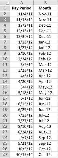
Since a PivotTable will “see” the underlying serial date, I’ll need to add another column for Month and give it a “Month-Year” format so the PivotTable will group similar Months together. For this I’ll use the TEXT formula. The "Pay Period" Date is used for the first value argument, and then “mmm-yy” for the format_text argument.
So the formula in cell B3 =TEXT(A3,"mmm-yy")
As you can see in the screen shot, the months Dec-11 and Jun-12 have three pay periods. A PivotTable will quickly summarize more than one year and show the number of times a pay period happens each month.
Add a PivotTable
The steps to create a PivotTable in Excel 2011 are as such.
- Select a cell inside the data range
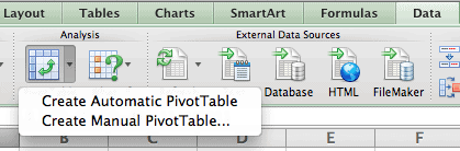
- Click the Data tab on the Ribbon
- Click the PivotTable drop-down arrow and select Create Manual PivotTable...
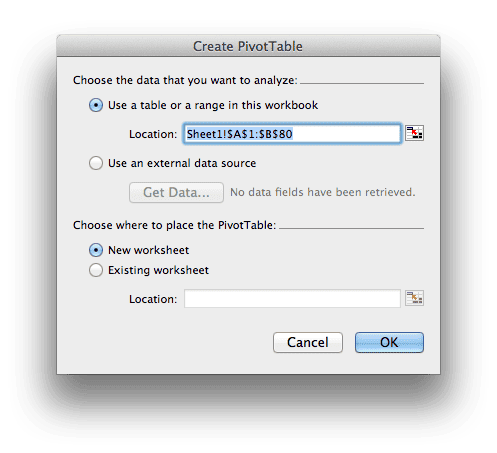
- On the PivotTable dialog box, click OK
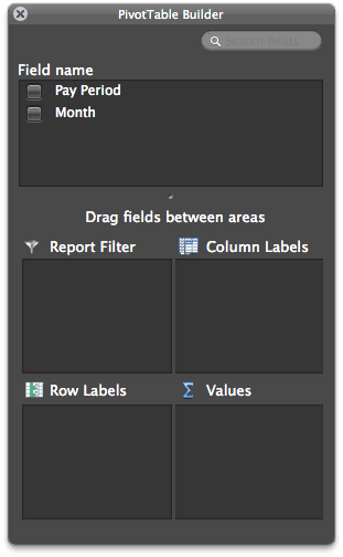
You'll get a new worksheet that shows an empty PivotTable Layout. There's an introductory PivotTable popup box that has a link to Learn more about PivotTables, which brings up the Help system topic About PivotTables. Click the x to dismiss this help box.
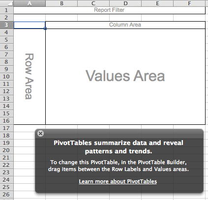
The PivotTable Builder box is also shown. This object looks quite a bit different from the traditional Windows counterpart. My first reaction was that it looks funky. Nevertheless, it's the functionality that counts.
Arrange the PivotTable Layout
Click and drag Month from the Field name area to the Row Labels area. Then click Month again and drag it to the Values area. (Yes that's right, you're dragging Month twice.)
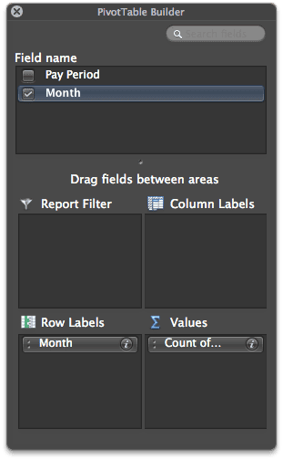
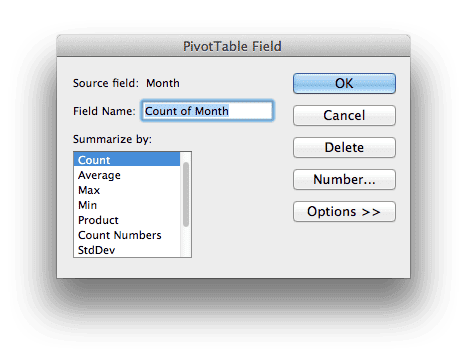
In the Values area you should see Count of... and to see the rest, just click the i to bring up the field name list.
Sort the PivotTable
Click inside the Data area (like cell B5) of the PivotTable and then select Descending from the Sort icon drop-down list on the Toolbar.
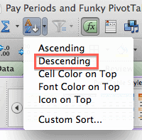
The top of the list shows months with 3 pay periods. Just what I was looking for.
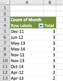
You'll notice the descending sort doesn't leave the Row Labels in ascending order. (Nov-12 doesn't follow Jun-12, etc.)
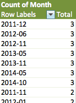
A Better Formula
You can change the Month formula to =TEXT(A2,"yyyy-mm") and the Row Labels will show up in year-month format in ascending order.
While this took some time to explain, the reality is when I do this it takes about two minutes. And the bulk of the time is generating the dates and adding the formula.