Category Archives: Formulas

All about formulas and functions

How To Calculate Hours Between Two Dates in Excel

Recently I was asked how to subtract time in Excel (time difference) or how to calculate the number of hours between two points in time on different days. Since this was in a reader comment, I gave a brief answer that requires a fuller account here.

Dates and Times are all part of the master plan in Excel. Once you “get” the fundamentals, the rest is just icing on the cake.

A Date value in Excel looks like this: 40519
A Time value in Excel looks like this: 0.58333

Cell formatting changes how you see these numbers.

The Date: 7 Dec, 2010
The Time: 2:00 PM

How to Calculate Time Between Dates in Excel or the Duration Between Two Dates

If you want to calculate time between dates in Excel or the duration between two dates, you need to understand what they mean first. When you type a Date into Excel, you may never see the underlying number, like 40519, but it’s there nonetheless. This is a date serial number and it makes Date calculations easy.

You might ask, “Why is this such a weird-looking number?”. Well, the Excel folks started a numbering system with Dates. In Excel for Windows they gave 1 Jan, 1900 the serial date number of 1, then continued numbering until this day and beyond. So serial number 40519 represents 7 Dec, 2010.

In Excel for Mac they started numbering Dates beginning with 2 Jan, 1904. (don’t ask) So the serial date 40519 represents 8 Dec, 2014 (Actually it’s known as the 1904 date system. To be clear, Macs can change Excel settings to use the 1900 date system).

How to Subtract Time in Excel (Time Difference)

When you type 2:00 PM into a cell in Excel the underlying value is a fraction, but Excel interprets this as a time serial number and formats the cell accordingly.

Try typing 0.25 into a blank cell, then change the cell formatting to a TIME format, and you’ll get something like 6:00 AM.

As an aside, you can calculate this fraction for any time value during the day by taking the total number of seconds that have passed from midnight until your time value and dividing by 86,400 seconds in a day.

Image of an equation to calculate time difference

Dates and Times Together

In Excel the unit of time is “the Day,” a key fact to know. You’ll notice that Dates are integers, and Time is a fractional number. You can add the two together to get a Date/Time format.

So adding a Date serial number, like 40518, to a Time serial number, like 0.25, gives us 40518.25. Formatting the cell holding this value using “d mmm, yyyy h:mm AM/PM” will show 6 Dec, 2010 6:00 AM.

You can also enter something like 7 Dec, 2010 2:00 PM into a cell and Excel will recognize this as a Date/Time format. However, if you change the cell formatting to General, the underlying number is 40519.05833.

So hopefully by now you can see that subtracting two Date/Time formatted numbers can be done mathematically. Subtracting 6 Dec, 2010 6:00 AM from 7 Dec, 2010 2:00 PM is done by Excel “underneath the hood” as 40519.05833 – 40518.25 and the result is 1.3333.

Calculating Hours Between Two Dates in Excel

If we recall that the unit of time is “the Day,” this value represents 1-1/3 days of time.  Since there are 24 hours in a day, converting to hours is a simple multiplication 24 * 1.3333 = or 32 hours. (24 * 4/3 to be more precise)

Time Between Two Times / Dates

Finding the number of hours or the time between two times/dates is simple, just subtract the start date/time from the end date/time and multiply the result by 24 hours.

If you want to enter the dates and times separately (which is loads easier than typing in a date/time in one cell) then add the date/times together.

Hours = ((End_Date+End_Time)-(Start_Date+Start_Time))*24

Here’s a look at a typical worksheet designed to calculate the hours between two dates.

Image of an Excel table with dates and times

As you can see, the formula for Hours, in cell F2, shows in the formula bar. And row 3 contains General formatting so you can view the date/time serial numbers for row 2.

Change the formatting for cells B2:E2 to match what you normally use for Date and Time data entry.

The NETWORKDAYS Function

People also asked how to calculate the time between days but without taking into account weekends or specified holidays. The NETWORKDAYS function will help you to calculate the time period by excluding weekdays and specified holidays.

The formula looks like this: =NETWORKDAYS(start_dateend_date, [holidays])

Like in the previous case the start_date and end_date are required arguments, yet the argument [holidays] is optional. You can use this argument to specify which days should be excluded.

Image of an Excel list showing NETWORKDAYS formula

This time I used two random dates which contained two weekends and I added two desired dates under the holidays argument just to show you how it works.

If you need to add some weekends you will have to add one more argument (weekends) and use =NETWORKDAYS.INTL(start_dateend_date[weekend][holidays])

After you calculated the days by using the NETWORKDAYS formula, to calculate the hours you can simply multiply the given number with the number of hours you need for as long as they stay the same.  Also, do not work harder by looking for complicated formulas to calculate simple things.

What else you should know:

  • If the start date is later than the end date the formula will generate a negative number.
  • The NETWORKDAYS formula will also include the start and the ending dates in the calculations, due to this if you have the same date the value returned will be 1.

If you want to find more formulas regarding the date and time feel free to check the following list of functions.

I hope this article helps you to better understand how to calculate hours between two dates in Excel. You can exercise what you learned today by calculating the time left until your next birthday, to do this you can also use the =Today function or the =Now function.

If you found this article helpful, please feel free to check our other articles about tips and tricks in Excel. We also have a dedicated section for details and formulas about dates and times in Excel.

image of excel showing the addition function

The Data Adds Up: Using the Addition Formula in Excel

Meta: In this article readers will learn the basic addition formula for Microsoft Excel. Users can find examples and a how-to guide for entering formulas themselves and using the sum feature.

The addition formula is one of the basic functions you can perform in Microsoft Excel and other spreadsheet programs. There are several different ways to use the addition formula in Excel and many different times when the formula will come in handy when you are working with data in your spreadsheet.

In the following article, we will discuss the different ways you can enter an addition formula, and when it is appropriate to use the formula. This will include sections on:

  • What is a formula in Excel
  • Basic addition formula
  • Advanced addition
  • The “SUM” function
  • SUM with rows and columns

What Is a Formula in Excel

In Excel, a formula is a way to perform calculations and other operations on your data. There are basic formulas such as addition or subtraction, which we will discuss in this article, and much more complex formulas that make calculations for advanced statistics or engineering problems. In essence, a formula is performing some simple, or complicated, mathematical function.

Any formula that you make in excel will begin with the “=” symbol and are most often entered into a specific cell of your choosing. For example, if you typed “= 5 + 3 + 8” into the cell A1 and pressed enter, what would you expect to get back? If you said 16, you’re exactly right. Pretty easy, no?

Values are not the only thing you can add using the addition formula. Formulas can also contain constants, individual cells (for example, B22) or a range of cells (for example, F2 to F22), functions, and operators.

In Excel, values are not limited to numbers. They can include dates, text or words, and Boolean values.

The Basic Addition Formula

Image of Excel showing formula bar with =2+2 and cell D4 showing 4
Screen capture from Excel: Cell D4 showing the result of the formula “=2+2” the formula is displayed in the formula bar

As we noted above, the basic addition formula is quite simple. Except for the syntax, you probably recognize it from your elementary school math class. In Excel, instead of writing “2 + 2 =”, you write = 2 + 2 and the program will spit back to you the number 4.

You can also write the names of cells into your formula instead of numbers and get the same result. For example, if you typed = A4+B4 into the C4 cell, the program would then do perform the function and give you the result in C4. In this case 4.

The huge advantage to using cell references rather than typing in the data is that if change the data in a cell, the formula will automatically change. This will cut down on making any errors when working with your data.

More Advanced Addition

As noted above, one way to do this is to type in the range of cell references you want. Above we did “=A4+B4” and got 4 back.

If you’re more of a mouse person, the other easy way to do this is the point and click method. Start by typing a “=” into C4. Now click on cell A4. This should show “=A4” in the cell. Then type the “+” sign and click on the cell you want to add to A4. In this example, we will do B4. Cell C4 will now have the completed formula “=A4+B4”.

addition formula for cells shown
Showing formula in cell C4

When you press enter, you will get the result, 4.

Excel screen capture showing c4
After hitting enter in C4, the sum of the selected cells is displayed, the formula shows in the formula bar above

If you need to change the formula, say you want to multiply the cells instead of adding them, double-click the cell containing the formula and change the “+” to “*” and press enter.

The Sum Function

In Excel, you don’t need to use the operator “+” to add together two or more numbers. You can also use what is called the SUM function. As with all formulas, you still start by typing an “=”, but now you type SUM and whatever numbers or cells you want added up.

For example you can type =SUM(2,2) into a cell.

Showing formula for cell C7 and total displayed in that cell

When you press enter you’ll get 4.

You can also type in cell references, for example, =SUM(A1, B1, C1). If you want to do a range of cells, type =SUM(A1:C1).

Showing range addition formula

The Sum Function for Rows and Columns

All of our examples so far have been pretty easy, and you might be wondering, why do we need such an easy formula when you can do it in your head?

Well, the more data you have in your spreadsheet, the longer it will take for you to do the addition by hand. Imagine you’re working in sales, and you have a spreadsheet that keeps track of units of your product you’ve shipped in the past year as well as the units that remain in your warehouse.

You could sit there and calculate the entire inventory by hand, but then what would the point be of recording everything in a spreadsheet?

To cut down on time without creating an elaborate formula to perform addition, you can use the “SUM” function. The SUM function is incredibly useful if you’re like our salesperson who wants to add up her sales from the previous year.

Annual sales shown for how to use the sum function (addition) in excel

In the example, you can see that we have a lot more data than in the earlier examples. By using the SUM function, we can easily add together all the data in a given column. You can do the same thing for a row, or for both rows and columns simply by typing in or clicking on the range you wish to add up.

You can later use this data to create pivot charts, or pivot tables.

Bringing it all Together

In this article, we introduced the addition formula for Excel spreadsheets. We discussed some of the reasons why you might choose to use the addition formula, types of values and references that can be added using the formula, and some of the shortcuts you can use to tell Excel to add data in your spreadsheet.

Person using a laptop with excel on screen

HLOOKUP In Excel: Everything You Need to Know

HLOOKUP is a tool that makes it easy to find the information you’re looking for without the hassle. You can search for specific data in any row of a table or spreadsheet quickly and efficiently, giving you the time to focus on more pressing issues. Using HLOOKUP can make your job just a little bit easier when using Excel.

Here, we’re going to go over everything that you need to know about the HLOOKUP function. We’ll be discussing:

  • The basics of the HLOOKUHow to use HLOOKUP
  • How to use HLOOKUP
  • When to use HLOOKUP

Let’s get started!

What is HLOOKUP

HLOOKUP is a handy search function in Excel that allows you to sort through large amounts of data effortlessly. You can isolate the information that you’re interested in based on specific criteria such as dates, numerical values, and text. HLOOKUP works by searching for and retrieving values from the first row in a table. As you may have guessed, the H in HLOOKUP stands for horizontal.

​How HLOOKUP Differs from VLOOKUP

If you’re familiar with using VLOOKUP in Excel, then you shouldn’t have too much trouble picking up the finer points of HLOOKUP. Both are search functions, but while VLOOKUP finds data on a vertical axis, HLOOKUP searches horizontally. The main reason to switch between VLOOKUP and HLOOKUP is the orientation of the data in your table or spreadsheet. If the data you’re looking at is categorized and organized along the horizontal axis, you should use HLOOKUP to find your results.

​How to Use HLOOKUP

HLOOKUP is a worksheet function, allowing you to bring up values directly on the table you’re currently using. The syntax you should use is as follows:

=HLOOKUP(lookup_value, table_array, row_index_num, [range_lookup])

This formula can be a little bit confusing at first glance, so let’s break it down into its basic components:

  • Lookup_value: The value that the function will search for in the first row of the table. This can be a number, text, or another cell.
  • Table_array: The range of cells you plan to search. You can either highlight cells or type in a reference to an array.
  • Row_index_num: This value is relative to the table_array that you choose. Instead of typing in a cell reference, you should type in the numeric value of where the row lies on your table. For example, you should input the first row as 1, the second row as 2, and so on.
  • Range_lookup: This is the only optional parameter when using HLOOKUP. It allows you to specify if you want Excel to search for an approximate value by typing in TRUE, or an exact value by entering FALSE. When this syntax argument is left out, the formula defaults to TRUE.

It’s best to use the FALSE range_lookup when dealing with text, as you’re looking for an exact result. This also allows you to use wildcard characters when entering your lookup_value. A question mark will let you search for any single text character, while an asterisk can match with a sequence of numbers. If you need to search for actual question marks or asterisks, you can simply add a tilde (~) before the character.

Person using excel HLOOKUP on a laptop
Image via Pixabay

​Common Problems

​While HLOOKUP can be an indispensable tool when used properly, just a single mistake in syntax can cause a major headache. If you’re having trouble getting the formula to work, don’t worry. Plenty of people have problems with Excel search functions, but they’re easy to tweak and troubleshoot so that you get the results you’re looking for. Here are some of the most common problems that Excel users face when it comes to HLOOKUP:

Results return as #N/A: Sometimes, HLOOKUP fails to find a match for a lookup_value. This is often due to the range_lookup that you use. If TRUE, an #N/A error has probably occurred because the smallest value in the lookup row is greater than the lookup_value. If false, then the error occurs because a match wasn’t found in the specified cells.

Results return as #REF!: This error generally means that the row_index_number is larger than the number of rows in your table, leaving the HLOOKUP formula without a proper reference.

Results return as #VALUE!: This error may occur because your row_index_number is less than one or nonnumeric. You may also see a #VALUE! error thanks to a typo in the [range_lookup] argument, since this parameter only recognizes TRUE or FALSE.

​Examples of Formulas

​There are plenty of useful applications for the Excel HLOOKUP function. It’s an invaluable tool in both business and at home that can help you keep track of large quantities of valuable information.

The formula is most commonly used in database maintenance, as it makes it easy to pinpoint specific points of data or information from a certain timeframe. HLOOKUP is an invaluable tool both in a business and home setting.

  • ​Get an approximate match: =HLOOKUP(lookup_value, table_array, row_index_num)
  • ​For an exact match: =HLOOKUP(lookup_value, table_array, row_index_num, FALSE)
  • ​Get the first text value: =HLOOKUP(“*”,range,1,FALSE)
  • ​Display “Not Found” in results instead of an error message: =IFNA(HLOOKUP(lookup_value, table_array, row_index_num, [range_lookup]), “Not Found”)
  • ​Using HLOOKUP from another workbook or spreadsheet: =HLOOKUP(lookup_value, sheetname!table_array, row_index_num, [range_lookup])

If you use a separate database in your HLOOKUP formula, it’s important to remember formatting. Worksheets with names containing spaces or non-alphabetical characters should be enclosed in single quotation marks. If you’re referencing another open workbook, you should include the name in square brackets. Closed workbooks need to have their entire path specified.

​Conclusion

Whether you’re an Excel expert or are just getting started, search functions can help you to complete your projects on schedule. Tools such as HLOOKUP make it easy to sift through data to find the information that’s relevant to your work. You can use HLOOKUP to help streamline operations at home and in the workplace.

We hope that our tutorial has helped you to better understand the many uses of the HLOOKUP function in Excel. By following the steps we’ve laid out, you can save time and frustration when searching through important databases.

Person in front of laptop with excel display

How to Create a Database in Excel

A database in Microsoft Excel makes it easy to input formulas and organize information. This is beneficial when doing everything from staying on top of business numbers to grading term papers. Whatever the reason might be, if you're looking at how to create a database in Excel you'll find all the information and answers you need right here.

Entering the Data Correctly

Whenever it comes to entering in formulas and creating databases it is very important for you to focus on entering the data correctly. it sounds simple enough, but the failure to enter even one number incorrectly (or even putting the decibel in the wrong location) can throw off the entire formula and skew the database.

You don't want to go back later and search through every single line of coding just to catch a single number that might be off. In many ways, it takes less time to just start from scratch instead of searching and trying to find these incorrect numbers. So, always take your time when entering information into the database.

Creating a Table

Excel on computer monitor

Image via pixabay.com

Creating a table in Microsoft Excel is rather straightforward. When you first open Excel you can select how many columns are in the database. You can always add more columns and rows later, so you're not stuck with a set number.

Just in case you're not sure, columns are the vertical bits of information. Every alphabetical identifier is a column. Rows, on the other hand, are horizontal. So every number is horizontal. when you create a table you will begin by creating an initial row. Each bit of information in these rows will be the heads of columns.

For example, if you're creating a table for student information (let's say you're a teacher), the first header might be the student name. The second header might be the student number, and the third header might be the student grade. Each of these headers are within the same row (horizontal). However, as "headers", the information are the tops of individual columns.

When creating a database, it is helpful to note that all rows are referred to as records, while all columns are referred to as fields. So, if someone is talking to you about the formation of a database and uses the terms records and fields, you will understand what they are referring to.

Adding Information

You can now begin to add information to your table. Follow the headers and type in the information under the appropriate headers (given the previous example, you'll type the student names under the name header, the number under the student number header, and the grade under the grade header).

Cells That Can and Cannot Be Left Empty

Person in front of silver laptop practicing how to create a database in excel

Image via pexels.com

When creating a database in Excel, you need to understand what cells can be left blank and what cells must have information. It is possible to leave full rows blank. You might want to include separate information under the main information of the database. You may have separate classes or other information in which you wish to keep portions of the database separate. You can do this by leaving one (or more) rows blank.

However, when it comes to how to create a database in Excel, you are not able to leave columns blank. All column information must come one after another. When you input codes and other information into the spreadsheet Excel will stop when it runs into full blank columns. So, if you leave a full column blank Excel will not look at any information to the right of this column. This is why you can't skip any columns or leave information blank.

Turning the Spreadsheet into a Table

spreadshee table cell

Image via pixabay.com

After you have the spreadsheet information typed upyou may want to convert it into a table within the file. This can be done in just a few short steps. First, you'll want to highlight all the cells you want to include within the table. Once you have done this click on the "Insert" button at the top of the program window. Now choose "Table." A pop-up window will ask you if the data for the table is correct (and if it has headers). Click "OK" and Microsoft Excel will create the headers.

Formulating the Database

Person writing on how to create a database in excel

Image via pexels.com

Now that you have the individual table within your Excel document it can be used as a database. However, you will need to know how to use the database and how to complete the formatting of the database to finish off the creation process. Once you know how to do this, you will complete the how to create a database in Excel exercise.

There are several tools available to you when it comes to how to create a database in Excel. It comes down to what exactly you want to do with your database. Should you want to move into the individual tools and format specific cells within your database you are able to click on the "Format As Table" drop-down menu and input whatever coding you might find necessary. You can also click on the "Format Cells" box, which allows you to customize the information in each individual cell.

The exact formula you use depends on the kind of information you are using and how you want it to interact with other cells within the database. There is no one specific kind of formula to use. There are literally thousands of formulas. You can also create your own mathematical formula, which is used to implement specific equations within the database. When entering in a formula through the "Format As Table" option, make sure the information is correct, otherwise, the entire formula will give you incorrect answers for what you're looking to accomplish.

Relational Database

Finger on block chain

Image via pixabay.com

Creating the relational database makes it possible to include several tables and spreadsheets into the database. To do this, after you have created the initial table you will want to press "CTRL" and "A" at the same time. This will highlight the entire table without clicking and dragging.

From here, the next step for how to create a database in Excel is you'll want to click the "Insert" button at the top of the screen and then choose "Table." Once this happens a new window will appear. Check off the box that reads "My Table Has Headers," then click the "OK" button. You will want to name the table in the new window that asks for the "Table Name." If you don't, Excel will name the table for you, which is nothing but a series of numbers and letters that are especially confusing (and will be difficult to track down later on).

Slave Tables

Macbook on desk

Image via pexels.com

There will be times where you'll want to create what is known as a "Slave Table," which can help with how to create a database in Excel. The slave table will include some coding or other bits of information that will influence the main table (and also carry out the requests of the main table).

In order to create the slave table (which you may find necessary when addressing the how to create a database in Excel question), you'll want to click the "+" sign found on the Navigation bar, then add two additional spreadsheets to the selection. After you have done this, name the first spreadsheet two spreadsheets. You will want to title the new slave table after one of the fields within your master table. This will make it possible to include more data regarding the original field in the slave field. It also allows you to edit information within the master field and have it copy over into the slave field without typing the changes a second time.

Now, you'll want to copy information from the master table and paste it into the slave table. For example, perhaps you only need the student name within the master table, but you want to provide more information based on the name in the slave table. Click inside of column A in the slave table and paster the information in. Add in whatever necessary information you might need in the slave table, then copy the entire table (you can click and drag or use the CTRL+A hotkey shortcut). Click "Insert," followed by "Table."

Within the slave table, there are bits of data that will influence what goes on with the master table. For example, if you have a grade point field within the master table, and a series of grades for a student within the slave table, whenever the numbers within the slave field are adjusted it will influence and change the information displayed within the master table. This way, you can always go into each individual student (as an example) and create slave tables to give you greater control over each table database.

How to Create a Database in Excel | Conclusion

If you want to utilize formulas within your spreadsheets, you will probably want to create a database in Microsoft Excel. By using this information you will learn how to create a database in Excel, which makes it easier to control the data you input. Once you have everything entered in you can always edit the data and alter the information to better fit your personal (or professional) needs.

The NOW Function in Excel: What It is and How to Use It

What is the Now Function in Excel?

For those new to all things Microsoft software, the now function in Excel continuously updates the date and time whenever there is a change within your document. You can either format the value by now as a date or opt to apply it as a date and time with a numerical format. The purpose of the function is to set (and keep track of) the date and time.

Notes on Use

While the Now function in Excel does not have parameters, it does require empty parenthesis. The value returned by the Now function automatically updates after each refresh. If you need to, you can use “F9” to force the worksheet to refresh, recalculate, and update the value. For those of you who need a static time (e.g. one that won’t change), you can use the keyboard shortcut “Ctrl + Shift” to enter the current time.

The NOW Function in Excel returns the current date and time − formatted as date and time − as shown below in cell B1. If the cell format was General before using the function, Excel will change the cell format to match your regional settings for date and time.

NOW Function in Action

The NOW Function has no arguments, but the empty parentheses () is required, as seen in the formula bar above.

NOW Function in Excel

The NOW Function in Excel is Volatile, meaning every time Excel calculates the worksheet the function result changes. And you can’t always tell when this will happen. To see what I mean, enter a NOW Function in a worksheet cell then play around with the worksheet.

I’m not a big fan of Volatile functions. Used sparingly they can serve a specific purpose, but left unchecked in a workbook with a large amount of data they can drastically slow things down.

The cell formatting in cell B2 is General and you can see the serial number. The integer to the left of the decimal point represents the date, and the numbers to the right of the decimal point represent time.

The B3 cell format is Date and you see only the date portion. The B4 cell format is Time and you see only the time portion. Both cells have the same underlying value, 40409.47966.

Tip for Static Date or Time in Now Function in Excel

To enter the current date into a worksheet use the keyboard shortcut Ctrl+; (semicolon). To enter the current time use Ctrl+Shift+: (colon). Both are static entries that won’t change.

how to subtract in excel

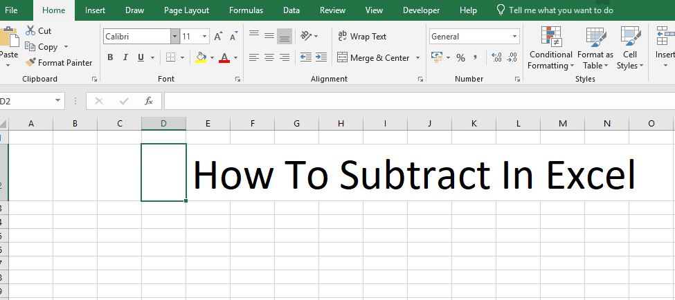
How to Subtract in Excel

Learn how to subtract in Excel with this valuable how-to guide. This article will walk you through each step of the process from start to finish.

Excel is a powerful program that makes organizing numbers and data easy for anyone. But, learning how to perform even simple functions can be a bit tricky when first starting out. Excel can perform many different functions and one of the most basic is subtraction. Below you will find a complete guide on how to subtract in Excel.

We don’t know why Microsoft didn’t make it but there is no subtract function in Excel. You don’t need to stress though. There are several helpful (and fairly simple) ways to perform this task on your own. Are you ready to improve your Excel skills? Learning new software methods, tips, and tricks is always helpful to have under your toolbelt. In this article, we have important points to remember, various types of Excel subtraction, methods for subtraction with two or more cells in Excel, and more. Read on to learn more.

how to subtract in excel

Important Points to Remember

Different Types of Excel Subtraction

As mentioned above, Excel can subtract numbers in a single cell or within a range of cells. Both operations are simple to perform and only a little different from one another.

Below, we will talk about the different ways to subtract in Excel and give you some examples.

To get the most out of the information below, keep these terms in mind while reading:

  • Worksheet: an electronic document made up of rows and columns that can contain data
  • Cell: the intersection of a row and a column on a worksheet
  • Formula: the instructions entered into a cell to produce a specific result
  • Function: a built-in formula used in Excel

Subtracting with Simple Numbers

For simple math problems, you can use a single cell to calculate subtraction problems. As an example, we’ll use the problem 5 – 4 = 1. This problem is simple, but you can apply the same concept to larger numbers and more complex data.

To begin, use your cursor to select an empty cell on the worksheet. Once you select the cell, begin to type your formula.

In Excel, all formulas start with an equal sign (=). After you’ve typed the equal sign, type the numbers you’re subtracting separated by the minus sign (-). In this case, your cell would contain the characters “=5-4.”

Once you have entered the numbers you’d like to subtract, hit the “Enter” key.

Hitting the “Enter” key tells Excel that you are ready to execute your formula. The data in the cell will transform from the formula you entered to the solution of that formula. The example cell would now read “1” instead of “=5-4.”

Subtraction Using Two or More Unique Cells

In Excel, every cell has a “name” made by combining its column letter with its row number.

This is the cell reference. For example, the cell created where column A intersects row 1 is cell A1. You can use cell references in formulas to execute various operations including subtraction.

Like before, this type of subtraction begins by selecting an empty cell.

Follow the same steps, but, instead of entering numbers, enter specific cell references. For example, if you’d like to subtract the quantity in cell A1 from the quantity in cell B1, your formula would read “=B1-A1.”

Instead of typing in a cell, you can also type formulas into the formula bar found at the top of the worksheet. You can also select cells with your cursor after starting your formula instead of typing them out.

How to Subtract Using the SUM Function

As mentioned earlier, functions are Excel’s built-in formulas. A variety of functions are available in Excel. When subtracting in excel, the SUM function is most useful.

Although addition and subtraction are often thought of as opposites they are, in fact, one and the same.

While we may not think about it, subtracting a number is the same as adding a negative number. Excel does not have a SUBTRACTION function but instead relies upon its built-in SUM function.

Excel’s SUM function can use individual numbers, cell references, or a range of cells.

To subtract numbers using the SUM function, make the number you want to subtract a negative value. For example, we’ll say that cell A1 contains the number 5 and cell A2 contains the number 3. You can use the SUM function in an empty cell to subtract 3 from 5.

First, make the number you want to subtract negative by adding a minus sign (-) to it. In this example, we are subtracting 3 from 5 so we will add the minus sign (-) to the 3 in cell A2 making it -3.

To use the SUM function, enter an equal sign into an empty cell followed by the word SUM.

The equal sign tells Excel that you will be using a formula. The word SUM specifies the function you want to use. In parentheses after the word SUM, press enter for the numbers, cell references, or range of cells in Excel you want to sum.

how to subtract in excel by first using the SUM function

For the example given above, your SUM function would look like one of the following:

  • If you used individual numbers, “=SUM(5,-3)”
  • For using cell references, “=SUM(A1, A2)”
  • If you selected a range of cells, “=SUM(A1: A2)”

In Excel, you can also use the AutoSUM wizard by clicking on the “Formulas” tab and then choosing AutoSUM. Always switch the values you are subtracting to negative when using the SUM function.

How To Subtract In Excel: Final Review

As you can see, there are several different methods for how to subtract in Excel. Depending upon the type of data you are dealing with, some of these methods will work better than others. You can use each method to subtract numbers both large and small and organize large amounts of data. Learning how to subtract in Excel is a quick and simple process that anyone can master.

With a small amount of patience, you can apply these concepts to any worksheet you come across. Subtraction may seem like an insignificant skill to gain, but it is a step towards harnessing the full power of Excel. Do you want to know more about Excel’s Intermediate features? If yes, then click here.

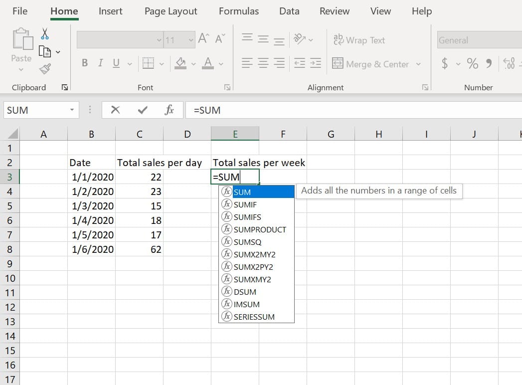
Excel SUM Formula: What Is It And When Do I Use It?

If you have a large database of information, it can be difficult to make sense of all those names numbers. The Excel SUM formula lets you focus on specific categories within an Excel worksheet and come up with subtotals that can help you to spot trends and patterns in your data.

Read on to find out more about:

  • How the SUM function works
  • Using the Excel SUM function
  • Different applications for SUM formulas

About the SUM Function

The SUM function is one of the simplest functions in Excel, but it’s also one of the most useful. It’s one of several math and trig functions available and allows you to add up multiple values. You can add up individual numbers, cell references, ranges of cells, or mix these values together. You can also use the SUM function as part of a more complicated order of operations to manipulate values. For example:

  • Addition: =SUM(A1:A10)+B1
  • Subtraction: =SUM(A1:A10)-B1
  • Multiplication: =SUM(A1:A10)*B1
  • Division: =SUM(A1:A10)/B1
  • Exponentiation: =SUM(A1:A10)^B1

How to Use the SUM Function

The Excel SUM formula is easy to use and easy to remember, even for complete beginners. The basic syntax of the function goes as follows:

=SUM(number1,[number2],…)

You only need to input a single range or value into the brackets, but if needed, you can include as many as 255 numbers. The parameters you’ll be using include:

  • number1: This value is required for the function to work properly. You can use a number such as 4, a cell reference such as A4, or a cell range like A1:A4.
  • number2-255: While you don’t have to input this value, if necessary, you can add hundreds of secondary numbers to your formula.

The SUM formula is a worksheet function, meaning that to use it, you simply type the appropriate syntax into a free cell to find out your end result. You can also use it in tables to total up rows and columns.

If you don’t want to display totals on your worksheet, you can find out the sum of a group of cells using the Excel status bar. Simply click and select the range, then look at the sum total listed in the lower right-hand side of the window.

Using SUM With Other Excel Functions

Excel has some built-in formulas that combine the SUM function with other useful tools. For example, combining SUM with the IF formula creates the SUMIF function, which allows you not only to add up data points, but also to choose these points based on criteria such as date, numeric value, text descriptors, and more.

You can also create your own formulas that combine the SUM function with other actions. Combining the operations of two or more functions is commonly known as “nesting functions.” There are endless ways that you can nest SUM with different Excel formulas. For example, you can combine SUM with the ROUND function to round decimals and fractions before adding them up, which can be handy come tax season.

Combining SUM with the VLOOKUP allows you to locate and sum values with that meet one or several criteria. No matter what the application, you can find a way to nest SUM with other Excel functions to get the results that you need.

Using Excel SUM Formula Across Multiple Worksheets

When using the SUM function, you might not always be dealing with values on a single spreadsheet. For example, if your company uses a different worksheet for each month or quarter, you may need to total data across several separate datasets. Instead of manually adding each relevant cell, it’s much easier to use a 3-Dimensional (or 3D) SUM.

The syntax to add a cell value from different sheets reads:

=SUM(SheetX:SheetY!cell#)

Common Problems With Using Excel SUM Formula

Although the Excel SUM formula is relatively straightforward, every now and then even the most tech-savvy of us run into issues. Here are some common problems you may run into when using SUM functions, and quick fixes to help save you a headache:

The result is displayed as ####: Often, this reading simply means that your column is too narrow to display the full result. Increase the width of your column to prevent this problem.

The formula won’t change to a result: The cell containing your SUM function may be formatted as a text cell, preventing the formula from working. Hit Ctrl+1 to bring up the Format Cells dialog, then click the Number tab to select the right format. You can also use F2 > Enter.

The function won’t update automatically: Open the Formula tab and go to Calculation to check that it’s set to automatic. You can also use the F9 key.

The #NAME? error appears: This usually means that a formula’s syntax is incorrect. Check to make sure that everything is spelled correctly and in the right order.

Examples of SUM Formulas

As an Excel user, you’re bound to run across the SUM function in various ways, shapes, and forms. Here are some of the more common formulas that utilize this tool:

When inputting individual cells or values:

=SUM(A1,A3,B2,C3…)

When inputting a range of values:

=SUM(A1:A3,B1:B3)

Sum an entire column:

=SUM(A:A)

Sum every nth row:

=SUM(OFFSET(A1,(ROW()-offset)*n,0,n,1))

Calculating a running total:

=SUM($A$1:A1)

Conclusion

excel shortcuts

The SUM function is a must-know tool for all Excel users, whether you’re just starting out or working with Microsoft on a professional level. The Excel SUM formula can help you to add points from complex sets of data and gain valuable insights that will help you or your company to make more well-informed decisions in the future.

We hope that our comprehensive guide has helped you to better understand the many uses of the SUM formula and hone your skills so that you can take full advantage of this invaluable tool.

average function in excel

How to Use the Average Function in Excel

Excel makes it easy to figure out the average of a group of numbers, no matter how large or small. It makes it easier for you to analyze important data. You will learn how to use Excel’s “average” function right here.

Most of us are familiar with average values. They offer a great way, to sum up information in a single number. Which gives us an immediate picture of any dataset.

If you have a large set of data, Excel can help you to find statistical values such as the average.

Not only can this help to enhance your understanding of a dataset, but it can also make information easier to present to supervisors, investors, and even loved ones. Using the AVERAGE function in Excel is easy and takes just a few clicks of the button.

In this tutorial, we’ll show you:

  • How to Use Average Values
  • Calculating Averages in Excel
  • Common Examples of the AVERAGE function

Using the average function in excel

What is an Average Function in Excel?

The average of a group of numbers describes the central value of the set.

The first thing to remembers is that using averages can help us to draw generalizations from sets of data.

There are three different ways that are commonly used to measure central tendency:

  • First is the Average: You can calculate the mean of a group of numbers by adding each value together and then dividing by the total count of those numbers. For example, in the group 2,3,5,5,5, the average is (2+3+5+5+5)/5=4. The average of a group of numbers is highly susceptible to outliers.
  • Second is the Median: The median is the number that lies directly in the middle of a set of numbers. For example, in the group 2,3,5,5,5, the median is 5.
  • The third is the Mode: The mode is the number that occurs most frequently in a set of numbers. In the example group of 2,3,5,5,5, the number 5 appears three times, making it the mode.

When Do Averages Come in Handy?

Averages aren’t just a part of your grade school math curriculum.

There are plenty of applications for averages in the real world, both at home and in the office. Notably, you can use averages to draw conclusions about your budget, your grades, yearly earnings, and even your car’s gas mileage too.

With this in mind, there are countless ways that averages can come in handy. However, you may want to look at different values depending on your situation.

The mean is best used with datasets that contain information that’s evenly spread, such as bell curves.

Extreme outliers in either direction can skew results and lead to false conclusions about central values in a dataset. It is important to realize that when outliers are in play, you should stick to using the median to represent the central value.

The mode works well for smaller sample sets. That is where there’s not enough data to draw relevant conclusions by calculating the mean or median.

The Basics of Excel’s Average Function

The AVERAGE function in Excel returns the mean number for any data set as opposed to the median or mode. In addition, it can be used as a worksheet function, making it easy to enter as part of a formula in a cell.

Your average will depend on the cells that you highlight. For this reason, it may be best to omit any statistically insignificant outliers. A value that’s too high or not high enough can skew your results, giving you an inaccurate picture of your dataset as a result.

Using the Average Function in Excel

Using the AVERAGE function is simple enough for even Excel novices to master in a matter of minutes. As a worksheet function, all you need to do is enter the formula correctly into a free cell to get a mean value.

The syntax you should use to find the arithmetic mean of a data set is:

AVERAGE (number1,[number2], …)

There are very few components that you’re required to input into this formula. There’s only one parameter that you really need to fill out in order to yield an accurate result.

  • Number1: This field is required. You can put in a cell value or a range of cells for which you want the average.
  • Number2: This field is optional. If you want to analyze additional cells or ranges, you can add up to 255 more to the AVERAGE formula.

If any of the cells in the range you highlighted contain text, logical values, or are simply empty, the AVERAGE formula will ignore these. Cells that contain a zero, however, are included. If you want to omit any cells within a row or column, you should leave them blank.

If the AVERAGE function isn’t coming up with the results that you’re looking for, then you may want to consider modifying the formula slightly.

The AVERAGEA and AVERAGEIF Function

The AVERAGEA function allows you to include logical values and text representations of numbers in a reference as part of your end result. This also gives you more control over formatting.

Moreover, you can also combine the AVERAGE function with the IF function to limit the range of values used to calculate a result.

Excel’s IF function allows you to see whether a data point meets a condition that you specify. For example, being greater than another number or occurring within a given timeframe.

The AVERAGEIF function gives you the power to calculate a mean using only values that meet certain criteria.

The Average Function in Action

Here are some examples of common formulas used to find the average of various sets of data:

  1. Single column – Average the last few values in a single column: =AVERAGE(OFFSET(A1,COUNT(A:A),0,-N))
  2. Different columns – Average the last few values in different columns: =AVERAGE(OFFSET(firstcell,0,COUNT(rng)-N,1,N))
  3. A range of numbers – Average the last few values in a range of numbers:

{=AVERAGE(LOOKUP(LARGE(IF(ISNUMBER(data),ROW(data)),{1,2,3…}),ROW(data), data))}

Average the top scores in a data set: =AVERAGE(LARGE(range,{1,2,3…}))

Conclusion

Ultimately, average values are an important part of everyday life. It helps us to quickly and easily understand even large datasets by giving us the central value of a group of numbers. Excel makes it easy to calculate mean values using the AVERAGE function.

Finally, we hope that this tutorial has helped you to better understand how to use the AVERAGE function in Excel.

Indeed the average function in Excel is such a powerful tool when it comes to analyzing data.

Do you need help in freezing columns in Excel? Here is a tutorial on how to do that.

excel sumif

How to Use the SUMIF and SUMIFS Functions in Excel

SUMIF and SUMIFS help Excel users to save time and frustration by making it easy to glean valuable information from complex datasets. You can total and analyze everything from grade values to quarterly earnings without giving yourself a massive headache.

In this tutorial, we’re going to cover:

The difference between SUMIF and SUMIFS functions.

How to use SUMIF and SUMIFS.

Common examples of formulas.

The Basics of SUMIF Functions

Most people are familiar with Excel’s SUM function, which allows you to add together highlighted data values in a row or column. The IF function is another favorite tool that lets you see whether or not a particular data point meets a specified condition, including dates, numbers, and text.

SUMIF combines both the SUM and the IF functions to bring you a tool that not only allows you to single out information that meets essential criteria but also to find the sum of qualifying cells. You can choose a single parameter to help you isolate relevant cells, combine the data, and pull totals to gain invaluable insights into the information that you've collected.

Using SUMIF Functions

SUMIF functions allow you to sort information based on one criterion, making it easy to pinpoint the data points you need. Like all Excel functions, though, you have to do a little bit of the work as well. To use SUMIF, you need to know how to express just what it is you’re looking for.

It is a worksheet function that requires a specific syntax to yield the best results. The basic syntax for the SUMIF function in Excel is:

SUMIF(range, criteria, [sum_range])

This formula may look a little complicated, especially for those just starting out with Excel, but once you get the hang of it, the function is relatively simple. There are only three different parameters that you have to keep in mind when using the SUMIF function:

Range: The cells that you wish to evaluate. It can be a column, a row, or randomly selected data points.

Criteria: The condition that must be met. Depending on your needs, you may wish to make this either text, a numeric value, or a wildcard value. It can even be another function. Just remember that all text or criteria including math symbols need to be enclosed in double quotation marks (").

Sum_Range: This parameter is optional, but it can help when dealing with particularly large data sets. It allows you to specify the range of cells you want to sum together. If you leave this element out of the SUMIF function, as many people do, the value will default to your (Range) parameter.

Examples of SUMIF Functions

sumif example

People use SUMIF functions every day in business, education, and in their personal lives. Here are some common formula examples that you might find yourself running across:

Subtotalling by a descriptor such as color: =SUMIF(descriptor_range,criteria,number_range)

Sum of cells that contain specific text: =SUMIF(range,"*text*",sum_range)

The sum is “less than”: =SUMIF(range,"<1000") The sum if “greater than”: =SUMIF(range,">1000")

The sum if cells are not equal to a specific value: =SUMIF(range,"<>value",sum_range)

Subtotalling invoices by age: =SUMIF(age,criteria,amount)

Subtotalling by invoice number: =IF(COUNTIF(range,criteria)=1,SUMIF(range,criteria,sum_range,"")

Summing up by group or label: =IF(A2=A1,"",SUMIF(A:A,A2,B:B))

Comparing SUMIF and SUMIFS

While the SUMIF formula allows you to differentiate between data based on a single criterion, SUMIFS will enable you to specify multiple parameters. This tool is a relatively recent development from Microsoft that only hit the markets in 2007, meaning that it's only available in Excel 2007 or higher. With SUMIFS, you can evaluate up to 127 criteria at once instead of just one. The function offers a much more powerful tool to categorize and analyze data.

When to Use SUMIFS Functions

SUMIF functions let you break down information based on a single differentiating factor, but that isn't always enough. Sometimes you need to narrow data down further to analyze it, and that’s where SUMIFS comes in. You can use comparison operators like equals, less than, greater than, less than or equal to in relation to other values to gain practical insights into the real world. The basic syntax for any SUMIFS function is:

SUMIFS(sum_range, criteria_range1, criteria1, [criteria_range2, criteria2], ...)

Unlike the SUMIF function, you’re required to input “[sum_range]” for SUMIFS. There are also other important parameters to define, including:

Sum_Range: The range of cells you wish to input and analyze. This field replaces the Range field used in SUMIF functions.

Criteria_Range1: This value is paired with Criteria1 to specify the range of cells to be searched.

Criteria 1: This defines the criteria that will be applied to cells in Criteria_range1. You can use text, numeric values, other cells, and even qualifying commands such as greater or less than. Any non-numeric criteria need to be enclosed in double quotes.

Criteria_range(#), Criteria(#): You can add up to 127 different criteria and range pairings onto the formula as needed.

Examples of SUMIFS Functions

using sumifs excel

Although SUMIFS is relatively new, it’s become common to see on both business and personal spreadsheets. SUMIFS formulas give users more precision and power when analyzing data sets. Here are some of the more common formulas that you might encounter:

Sum by week number: =SUMIFS(sum_range,weekrange,week)

The subtotal falling between two dates: =SUMIFS(amount,start_date,">"&A1,end_date,"<"&B1) The sum of sales based on ID and time frame: =SUMIFS(amounts,dates,">="&TODAY()-30,ids,id)

Conclusion

Excel is an invaluable tool when it comes to data analysis. Functions such as SUMIF and SUMIFS make it easy to break down information by allowing you to subtotal data based on essential criteria.

We hope that this tutorial has helped you further down the path towards becoming an Excel master. The next time that you have to subtotal data don’t forget to take advantage of the SUMIF and SUMIFS functions.


Related Posts Plugin for WordPress, Blogger...