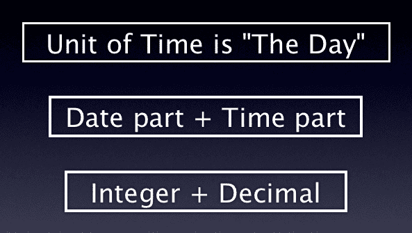
The unit of time in Excel is the Day. By using the NOW Function to show both date and time, you can see the underlying serial number by changing the cell format to General.
This serial number is composed of two parts: the date part is the integer and the time part is the decimal.
The Date serial number is an integer value based upon a Date System, either Windows or Mac. The Time serial number is represented as a decimal fraction because time is considered a portion of a day.
The Date and Time Calculator (Excel)
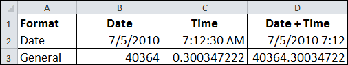
In the table below I entered a date in cell B2, a time in C2, and a formula in D2 that adds the two together. Excel automatically formatted this cell using a m/d/yyyy hh:mm format. I changed the row 3 cell formatting to General so you can see the serial number values. This is the function for time calculator in Excel.
You can clearly see that Date is a integer value, Time is a decimal fraction, and the Date/Time format has both together in one number.
Date and Time Calculations
In Excel, date serial number 1 is Jan 1, 1900 for the Windows Date System. The date serial number 40364 represents July 5, 2010 because it's 40,363 days after Jan 1, 1900. These date serial numbers are used in calculations by Excel.
Time is a decimal value from zero (0) to 0.99999999, representing times from 0:00:00 (midnight) to 23:59:59 (11:59:59 pm).
Think about time values as the number of seconds past 12:00 AM divided by the number of seconds in a day, 86,400. Obviously this can be simplified if using only hours or minutes. For example, the time value for 6:00 AM is 0.25, which is 6hrs divided by 24hrs.
The time shown above (7:12:30 AM) has a decimal value of 0.300347222. The calculation is:
7 hours = 7 hrs x 60 min/hr x 60 sec/min = 25,200 seconds
12 minutes = 12 min x 60 sec/min = 720 seconds
Total seconds = 25,200 + 720 + 30 = 25,950
Decimal value = 25,950 / 86,400 = 0.300347222
Change the cell formatting to Time and you will see 7:12:30 AM (or your local Time setting format).
Tip: When subtracting two different times not in the same day, the integer portion of the serial number must be used or the calculation will be invalid.
Enjoyed this guide?
Join our newsletter to get the latest Excel tips delivered to your inbox.
Comments migrated from the previous version of the site. Adding new comments is disabled.
bperumalOctober 17, 2010 at 03:44 AM
xls format
Misty MartinezDecember 7, 2010 at 09:44 PM
I need to find out if you can help me with a formula to conduct a spreadsheet calculating the number of hours between 2 different dates and times? Is this possible?
Construct a spreadsheet as follows: Cell A1 = Date 1, cell A2 = Date 2, cell A3 = Hours. (the labels)
Format cells A2 and B2 by selecting the cells and using keyboard shortcut Ctrl+1 to bring up the Format Cells dialog box, select the Number tab, and under Category: click Custom, then type m/d/yyy h:mm AM/PM into the text box below Type: and click OK.
In cell C2 enter the formula =(B2-A2)*24
Date 1 has to come before Date 2, so enter something like 12/6/2010 6:00 AM into cell A2, then enter something like 12/7/2010 2:00 PM into cell B2, and you'll see cell D2 show the value 32. I formatted this cell in a Number format with showing one decimal place.
I'll write a post about this on Thursday to explain why this works and an easier way to enter the date and times. Hope this helped.
Misty MartinezDecember 7, 2010 at 10:35 PM
what if i need the date and time in 2 different boxes
ex--A1 start date B1 start time C1 end date and D1 end time
Will this formula still work?
You have to add the date and time together to get what's known as a serial date. So given your example, the formula is =((C1+D1)-(A1+B1))*24 to get the number of Hours. In words that's ((End Date + End Time) -(Start Date + Start Time) ) * 24 hours.
JEETFebruary 11, 2011 at 10:59 AM
it work only when you have to calculate within 24 hrs
You bring up a good point about calculating time between two different dates. I will write a post about this issue next Monday. For now you can refer to the article I wrote: Calculate Hours Between Two Dates and Times in Excel.
Misty MartinezDecember 7, 2010 at 11:22 PM
YOU ARE AWESOME!!! THANK YOU SO MUCH
EnayatDecember 9, 2010 at 07:19 AM
Hi,
How to calculate hours which falls between two days as follows:
From Sunday 12:00AM To Monday 12:00AM which should be 24 hours.
If it is from Sunday 12:00AM to Sunday 11:59PM,the formula in the cell formatted as hh:mm results correctly. For Example: 11:59PM - 12:00AM=23.59 but from 12:00AM to 12:00AM which is expected a total of 24 hours confuses me how to apply to formula since the times don't refer to the same day or date.
12:00am - 12:00am+1 or *12 also doesn't work!
Thanks for your quick solution.
What you're trying to do includes two different dates. It just so happens that tomorrow I'm posting an article on how to calculate the number of hours between two dates and times. Suffice to say here that you have to include the serial date with the time, and then subtracting the two will give you an answer in days 1.
What you propose is actually the same thing that happens when you subtract two dates like 9 Dec, 2010 minus 8 Dec, 2010 which would equal one (1) because the default time for every date is 12:00 AM, that is technically 00:00:00. Since the unit of time is "the Day" and there are 24 hours in a day, your answer is 24 hours.
All will become clear in tomorrow's article. Until then read the comments for this article where @Misty wanted to know how to calculate time between two different dates.
EnayatDecember 11, 2010 at 03:59 AM
Your are great! Mr.Gregory,
According to your comments, we must enter the date along with the time, right?
I tried your formula and it is almost what I wanted. I am trying it in different situations to see if it is applicable.Will be back in case further help is needed.
Thanks a lot.
I was completely off-base with my previous answers. All you have to do is format the (B-A) cell with a custom time format [h]:mm.
JEETFebruary 11, 2011 at 10:56 AM
A-02.02.2011 10:00
B-05.02.2011 17:00
Please help me to find B-A in hh:mm
Santhosh ShettyMarch 8, 2012 at 11:47 AM
Hii i want to calculate the Time difference.
Input Values are
Start Date 13-Mar
Start Time 2.30 pm
End Date 15-Mar
End Time 10.05 am
total time ???????
The formula is: Hours = ((End_Date+End_Time)-(Start_Date+Start_Time))*24
to get a number in hours. I wrote about it in this blog post. You get 43.583 hours.
Another way to do this is to let Excel interpret the time and change the cell time formatting to reflect hours and minutes. To do that enter this formula: (End_Date+End_Time)-(Start_Date+Start_Time) and you'll get 1.8159722 for a result, it's a serial date/time. Next use Control+1 (or Command+1 on a Mac) to bring up the Format Cells dialog box, select Custom in the Category pane, then in the Type: box enter [h]:mm and click OK. The cell will show 43:35 which is 43 hours and 35 minutes.
Santhosh ShettyMarch 23, 2012 at 04:40 AM
Thanks its very easy!.. ;lOnce again thanks for the updating regading time related issue!...
chrisMarch 22, 2012 at 07:58 PM
Hi, I'm not sure if this is the right place, but I am working in a table and have a date field with hours and minutes: 11/17/2011 8:48:44 AM. I'm trying to create a new column to return the same value but with the times removed, so the result is 11/17/2011. Know of a way to do this? Day just gives me "17," but I want the month and year too.
@ chris, Assume your date/time (11/17/2011 8:48:44 AM) is in cell A2. You can get the date a couple of ways. 1) Enter the formula =DATE(YEAR(A2),MONTH(A2),DAY(A2)) and this will give you the date only. 2) Enter the formula =INT(A2) and change the cell formatting to Date.
chrisMarch 23, 2012 at 04:33 PM
Gregory, this was tremendously helpful. Thank you!
Santhosh ShettyMarch 23, 2012 at 04:42 AM
Hii How to put password for the defined cell or a column.
There are two things you have to do to password protect a defined cell or column. Lets start with step 2, protect sheet. There are two option when you protect a sheet or cell, or range. You can allow users of the workbook to either 1) select unlocked cells, or 2) select both unlocked cells and locked cells. To see these options depends on the version of Excel you are using. For Excel 2010, 2007 (Windows) you choose Review from the Ribbon, then click Protect Sheet. In Excel 2003 (Windows) and Excel 2011 (Mac) you choose Tools > Protection > Protect Sheet. The protection works even if you don't set a password.
Now, the cells or range you want to protect has to be selected and you then right-click and choose Format Cells from the pop-up box, and click on the Protection tab. Here you have an option for Locked. The default is that this box is checked. Meaning that all cells in the worksheet will be locked if you password protect the sheet. If you uncheck this box, the cells you selected will be available to users when you protect the sheet. All other cells will be locked to them after you protect the sheet.
Then you go back and protect the sheet. If you use a password, make sure you remember it. Otherwise you'll have a big problem.
Santhosh ShettyMarch 24, 2012 at 07:20 AM
In 2010 excell having pivot version is different than the earlier. I changed to old version but i dont know how i done.. In old version after clicking piviot wizard the header value is pasted in left column but in new version same header value is pasted in right side column ansd same is automatically get updated in left side column. Pls suggest how to go about old version which is very easy..
@Santhosh Try this: Right click on your pivot table, select PivotTable Options from the pop-up menu, click the Display tab, then check the box: Classic PivotTable layout (enables dragging of fields in the grid).
SitiJune 8, 2012 at 03:44 AM
dear,
How am I to put hour and minutes word in the formula?
Eg :43.58 become 43 hour 58 min
thank you in advance
Assuming your number 43.58 is using the period as a decimal number and not a time format, and assuming the value is in cell A2, here's a formula that includes the text you want.
=INT(A2) & " hour " & ROUND(MOD(A2,1)*100,0) & " min"
SitiJune 8, 2012 at 06:31 AM
Thanks Gregory, how ever I still cannot get it..
Let try one more example if I want to calculate overtime (all in HH:mm format)
17:30 until 20:00 = 2:30, I want 2:30 become 2 hours 30 min
if I'm using your formula, its not work because I'm using HH:MM format.
Select cells B2 and C2, right click the selection and select Format Cells from the pop-up menu. Select the Number tab in the Format Cells dialog box, and under Category click Custom and type hh:mm:ss then click OK. Now these cells show the hours:minutes:seconds.
If 3:30 is Hours:Minutes, then type in 3:30 into cell B2. Then in cell C2 enter the formula =B2+A2 and you'll get 12:13:30 as your answer.
If 3:30 is Minutes:Seconds, the type in 0:3:30 into cell B2. Then in cell C2 enter the formula =B2+A2 and you'll get 8:47:00 as your answer.
TimothyAugust 2, 2012 at 12:19 PM
To whom may be able to help,I have a work spreadsheet with detail of the parts I order .
It contains several formulas in hidden columns which tell me how many days since the order was placed and shades cells when the order is recieved etc etc.
Can you tell me of a formula which will highlight a cell in the part number column if the same value is entered say within 7 days?( to prevent me ordering the same thing too soon).
The sheet has a manually entered date for the date ordered and a column with todays date ....a formula subtracts one from the other telling me how many days since it was ordered.
Hope you can help...Tim
You can use conditional formatting to accomplish this task in a couple of steps. Assume Part Number is in column A, Start Date in column B, Today's Date in column C, and Delta Days in column D. Further assume the headings are in row 1 and the data starts in row 2.
To create conditional formatting for Part Number, select the Part Number date and choose Conditional Formatting (this varies by version of Excel.) You have to enter a formula, so navigate to this within the conditional formatting dialog box (again the navigation is different in each version of Excel.)
The formula you want is for the top row of your selection, in this case row 2. Hence my formula is =D2<8 and then select the formatting you want, then click OK. What this formulas does is look to the number of days and if it's less than 8 (0 to 7) then the condition will be true and the formatting will occur. It's important to open the conditional formatting dialog box and make sure Excel didn't add an absolute reference, like =$D$2<8 with the dollar signs. If this happends remove the dollar signs and your all set.
Hope this helps.
SamAugust 7, 2012 at 07:23 PM
I want to display a time interval in my excel spread sheet that looks like this
5:00 PM - 5:15 PM
So, that if I type in the time, 5:00 PM, for example what will come out in another cell is
5:00 PM - 5:15 PM
I have tried on my own and I keep getting the time in the decimal format. Please help.
Sorry for the delay in responding. Assume you enter 5:00 PM into cell A1. Then in cell B1 you would type in the following formula:
=TEXT(A1,"h:mm AM/PM") & " - " & TEXT(TIME(HOUR(A1),MINUTE(A1)+15,0),"h:mm AM/PM"
When you combine the two times with a hyphen between them, you end up with a Text cell format. Therefore you have to use the TEXT formula that will provide the formatting you specify in the second argument. I had to use the TIME function (with HOUR and MINUTE embedded) so I could add 15 minutes to the first time value, and then use the result as the value for the TEXT function.
matthewAugust 15, 2012 at 02:11 PM
Hi, is there a way in which I can simply type in a time value in one column (example a an event which begins at 9:30AM) and then have it calculate another time in a different column some time earlier (example: 2nd column shows up two hours earlier as 7:30AM). I am basically looking to type in one time and them the other column shows an earlier time (like a work shift which begins some time before an event executes).
Thankyou in advance for your assistance!
Assume you have 9:30 AM in cell A2. You can type the following formula in cell B2, which will give you the time 7:30 AM or 2 hours earlier.
=TIME(HOUR(A2)-2,MINUTE(A2),0)
Use the TIME Function, which has three arguments: Hour, Minute, Second. You have to use HOUR and MINUTE Functions to convert the time in cell A2. The last argument for Seconds can be zero (0). You simply subtract 2 inside the first argument for Hours (but not inside the HOURS function). If you wanted to subtract 1 hour and 30 minutes, which is 90 minutes, the formula would be:
=TIME(HOUR(A2),MINUTE(A2)-90,0) which would give you 8:00 AM.
Hope this helps.
DenitaAugust 28, 2012 at 02:21 AM
I have temperature data for every hour of the year for my research. I needed to convert AM/PM time to military time. When trying to format cells or copying into a new cell and format, it always gives me the (1/1/1900 12:45) in the same cell. I have also tried manually typing in the first few and dragging down, but it resets to that format for every 24-hour period. To complete the sorting I need to do, I can't have that date in the cell. I have no idea how to remove it at this point aside from manually doing it to 8000 cells x 8 field sites. Do you know of a much more practical solution to this problem?
To rid yourself of the "date" component of the date/time serial number, you only need a formula. Assume you have your date/time of 1/1/1900 12:45 in cell A3. I entered the following formula in cell B3:
=TIME(HOUR(A3),MINUTE(A3),SECOND(A3))
and that rids you of the Year portion. You end up with 12:45.
Now you can copy the formula down the column. This can be done simply by selecting the cell with the formula, and double clicking the bottom-right corner, which is called the "fill handle." Next you can select the entire range with the formulas, then Copy and Paste Special as Values to rid yourself of the formula and leave only the new values.
Hope this helps.
DenitaAugust 30, 2012 at 03:18 AM
You just made my day off so much more productive. Thank you!
AngelSeptember 28, 2012 at 06:02 PM
Okay, Maybe I'm just confused. I just want to add hours, as if compiling hours for a time sheet. So, how can I had the hours from 6:00 AM to 6:00 PM, etc. I tried the formatting and I'm pretty sure it's just something silly that I'm doing. Thank you.
Then use =(B1-A1)*24 and you get 12.75 which the difference on time multiplied by 24 hours.
45 min = .75 hours.
Make sure you change the cell formatting to General.
CindyOctober 1, 2012 at 04:41 PM
I'm trying to organize a teleconference of people who are in different time zones (one hour behind me to 16 hours ahead of me). Is there a formula that will tell me what time it is in someone's location based on a time and date I enter for my location?
Not that I'm aware of. However, I believe timeanddate.com has something like that for meetings across time zones.
CindyOctober 1, 2012 at 05:30 PM
I actually figured it out by playing around with it a bit more. All cells are custom format m/d/yyy h:mm AM/PM.
Cell A1 = my location date and time
Cell A2... = the cities of my committee members
Cell B2... = difference in hours between me and the members e.g. -1, 0, +14, etc.
Cell C2... = $A$1+(B2/24)
You have to put in the - and + signs to calculate the hours properly. It calculates the change in dates if you move into the next day. So all I have to do is change the time and date in Cell A1 whenever I need to schedule a teleconference. Handy!
From your earlier comment, I didn't realize you had all the cites and time differences figured out. Glad to see you've put it together, especially with the change in dates. Good stuff.
CindyOctober 1, 2012 at 06:25 PM
Oh yes, I forget to say that I knew the time differences. It was easy enough to figure out the times in my head, but I didn't want to change the dates and times every time I have a teleconference. Figuring out the formula makes it easier to try and schedule a time where people don't have to wake up at 3 a.m. to participate. Thanks!
SitiNovember 1, 2012 at 11:41 AM
Dear,
How to get the sum of hour and minute if i have the following data,
From To total H & M
17:30 20:00 2 hour 30 min
15:30 20:00 4 hour 30 min
14:30 20:00 5 hour 30 min
14:30 20:00 5 hour 30 min
14:30 20:00 5 hour 30 min
14:30 20:00 5 hour 30 min
14:30 20:00 5 hour 30 min
Grand Total .............. 0:00
I try to click the sum button but grand total will appear "0:00"
Need your help.
Thank you in advance.
Assume you have the start time in range A2:A8, and the end times in the range B2:B8. Assume the duration is in the range C2:C8 and it's a text field as you have depicted in your comment (2 hour 30 min, etc.)
To sum the difference for all the entries, in cell C9 you can enter the formula =SUMPRODUCT(B2:B8-A2:A8). However this is only half the battle.
Next you have to use a custom time format for cell C9, which is [h]:mm;@. This is just a regular time format, but you have to add the square brackets around the hour [h] so that Excel will summarize the cumulative time. If you leave off the square brackets it you will always get a number of hours between 1 and 24. The total is shown as 34:30 when using square brackets, which is what you are after.
SitiNovember 5, 2012 at 01:17 AM
Thanks Sir.=)
FIONANovember 20, 2012 at 07:15 AM
Hi Gregory
I have a mixed date/time field imported from other software into excel and it imports it as a serial number such as
20121116111903000
We need it to look like dd/mm/yyyy hh:mm:ss AM/PM. We are using version 2003 excel and have tried the custom format but without success. It remains a serial number.
Thanks for your assistance with this frustrating issue.
The number in your example, 20121116111903000, is not a date/time serial number. It's simply the date and time exported without any demarcation. That is no colons(:) between the time elements and no slashes (/) between the date elements.
The format appears to be YYYYMMDDHHMMSS000 for the export. From left to right you can see that 2012 is the year, 11 is the month, and 16 is the day. The time appears to be 11:19:03. The actual date/time serial number for this would be 41229.47156.
You can separate these components with the LEFT and MID functions, but those functions return a Text value, so you have to wrap either of those functions into the VALUE function. Then each of those different parts need to be used as arguments for either the DATE function, or TIME Function. And finally you have to add those two functions together to get the result you want. Very cumbersome.
You can break this down into parts to make is easier, which is most certainly what has to be done. However, I did this and it took up 9 cells to get the answer. Assuming the number is in cell A2, the following formula would pull out the Year: =VALUE(LEFT(A2,4)) and a formula for the Month would be =VALUE(MID(A2,5,2)) and a formula to pull out the Day is =VALUE(MID(A2,7,2)). Then you can pull out the Date with the formula =TIME(E2,F2,G2) assuming the Year, Month, and Day formulas just mentioned are in cells E2, F2, and G2, respectively.
The best solution is to try and get the export data in a recognizable Date/Time format. It should be a simple matter, considering the hoops you have to go through with Excel. I'll send you a worksheet that will pull out the date/time with this type of export data, but it's only a stop-gap measure. You need better export data.
AUSDecember 11, 2012 at 08:55 AM
Dear Gregory,
i've crack my head just to think of this calculation. to make it simple, assume that i have this time in "A" Column read as d:hh:mm and "B" Column with business day(note that 1 is consider as 8 hours)
1:22:53 4
0:02:45 2
0:00:02 1
0:00:07 1
0:01:47 2
"A" column is like timer is in 24hrs format as u can see from it counting above whereas "B" Column in business day. i'll be guessing that i will required to change the "A" column format to business day first before i could minus it.
i just want to get the business day in "B" to minus the time in "A" and get the result in business day.(8 hours)
Please help....X_X
Using the first row, multiply 4 business days times 8 hours to get 32 business hours. The designation of d:hh:mm for 1:22:53 as 1 day 22 hours and 53 minutes is where the tricky part comes in. Excel recognizes this number as h:mm:ss or 1 hour 22 minutes and 53 seconds, so we have to convert this number to hours.
Assume 1:22:53 is in cell A2, and a formula to convert to hours is =HOUR(A2)*8+MINUTE(A2)+SECOND(A2)/60 which results in 30.833 hours. Subtracting the two numbers 32 - 30.833 and multiplying the result by 8 business hours per day, gives you 3.86 business gives 0.14 business days.
The second row results in 1.66 business days.
Hope this helps. :)
AUSDecember 12, 2012 at 07:28 AM
dear gregory,
i get the amount 30.833 where i move the decimal places to 4 in "number" format. however, i did not get the amount of 3.86 nor 0.14 and also 1.66.
i put in at C2 this formula to make it simple. =(32-B2)*8 where B2 is place i put the formula =HOUR(A2)*8+MINUTE(A2)+SECOND(A2)/60.
However, i've think of other alternatives for this but still screwed up. Please ignore the previous request and this is the new one. Using almost the same table, i would like to minus today date at 8.30 AM and noon 12.30 PM.
1:00:00 12/12/2012 8:30:00 AM
1:22:53 12/12/2012 12:30:00 PM
0:02:45 12/12/2012 12:30:00 PM
0:00:02 12/12/2012 8:30:00 AM
0:01:47 12/12/2012 8:30:00 AM
i was hoping the answer in C2 to be 12/11/2012 8:30:00 AM and so on for the others. oh and still, under column "A" is supposed to be dd:hh:mm.
Please help and sorry for any inconvenience caused....
NickDecember 17, 2012 at 02:10 PM
I am a dispatcher and I need to be able to enter times in the format (1354) to represent (13:54). I need help formatting my cell to allow this, and then I need to be able to calculate total number of hours (Sometimes my drivers work into the next day, they may start at 13:54, and get off the next day at 4:32). Can you help me?
Nick
Assume Start Time of 1354 in cell A2 and End Time of 432 in cell B2. The formula to show the number of hours and minutes is:
=IF(B4>A4,TIME(INT(B4/100),MOD(B4/100,1)*100,0)-TIME(INT(A4/100),MOD(A4/100,1)*100,0),TIME(INT(B4/100),MOD(B4/100,1)*100,0)+1-TIME(INT(A4/100),MOD(A4/100,1)*100,0))
which gives you 14:38 hours and minutes when the cell is formatted in h:mm time format. You can multiply that number by 24 and change the cell formatting to General to get 14.63 hours.
HedayatDecember 18, 2012 at 12:21 PM
how to add this data h:mm:ss, looks so simple but it gives wrong result.i want total hours(i.e h:mm:ss format).kindly help.
0:12:23
0:27:22
1:28:31
1:25:46
1:28:41
0:55:38
0:12:42
1:20:21
0:38:57
0:47:5
1:44:24
0:26:33
0:49:32
0:27:57
1:51:54
0:11:06
1:37:56
0:43:28
0:15:53
Simply sum the cells in the range that holds the time data, and then make sure the cell format for the summary cell is [h]:mm:ss which will allow the hours to accumulate properly. The square brackets around the hours is the key. You can do this in the Custom tab of the Format Cells dialog box.
SitiDecember 28, 2012 at 02:12 AM
Hi Gregory,
How we want to convert time in 12 hour format to become 24 hour format.
I try to use custom format but it does not work.
The custom format hh:mm will give you the 24 hour format. Or you can choose Time in the Format Cells dialog box and select a time format that does not have AM or PM, which will give you a 24 hour format.
Santhosh ShettyDecember 31, 2012 at 07:31 AM
I need to convert 5.45 PM time in 24Hr format.
Pls help!..
Many Regards
Santhosh Shetty
You need to change the cell formatting. In cell A1 type in 5:45 AM, then in cell B1 type in the formula =A1 which will give you two cells with 5:45 PM. Select cell B1 and use the keyboard shortcut Ctrl+1 ( or CMD+1 on a Mac) to bring up the Format Cells dialog box. Click on the Number tab and select Time in the Category pane. You should see a few formats that don't have an AM/PM, which you should select and click OK. (My choice was 13:30 which may or may not match what you will see.) YOu should now see 17:45 in cell B1.
Another way to show the 24 hour format is to change the cell formatting by using the Custom format and type in h:mm for hours and minutes.
Santhosh ShettyJanuary 1, 2013 at 03:29 AM
Dear Gregory,
Wish you & your family a very happy & prosperous new year - 2013.
Thanks for the rply. Its working in the case time is mentioned in 5:45 PM format. But my time value is in the format 5.45 PM (.).
Best Regards
Santhosh Shetty!.
AravindMarch 20, 2013 at 09:52 AM
Hi,
I want to calculate the numbers hours spent for a particular work.
I have the date and time in each cell as mentioned below
(3/18/2013 9:38) and (3/20/2013 12:20)
when i do minus both i.e {(3/18/2013 9:38)-(3/20/2013 12:20)} the answer should get be 51 hours 42 mints, but in excel cell it is display's as 2:41:37.
mean it only considering the single day hours.
Help me out pls........
EnayatMarch 25, 2013 at 09:05 PM
Dear Aravind,
There are many useful methods but the one I just tried with the result what you exactly wanted is below:
Pretend your start-time is located in Cell A1 and End-Time in B1.
A1>>> 3/18/2013 9:38:00 AM
B1>>>3/20/2013 12:20:00 PM
Formula: =(DAYS360(A1,B1)*24+1)+HOUR(MOD(B1-A1,1))&":"&MINUTE(MOD(B1-A1,1))
First you need to find the number of days by function Days360 and Multiply it by 24Hours to find exact Hours based on number of days. Note: From 18th to 20th the result will be 2 days, while it should be three days e.g (18th,19th and 20th) therefore it should be +1. I think there is no need to explain the rest of the formula.. at a glance you can pick the meaning of the formula.
Hope you find it helpful,else, there are many respectful experts to guide you properly.
Regards,
Enayat
SitiApril 11, 2013 at 02:52 AM
hi, Enayat,
I try to use your solution for Aravind problem due to I am also facing the same problem.However it does not work.
Currently I am facing the problemto calculate overtime for working shift people which is Overtime start on :
eg :
01 Apr 2013 9:30 pm until 1:30 am 02 April 2013 = 4 hours
How to calculate the total hours with different date.
Please help.
thank you inadvance.
I need to find a was to capture the date and time difference.
Eg: 01/04/2013 8:00am - 02/04/2013 09:00 i need to find the difference also don't want to capture the full day. just the business hours which is 8am-5pm.
So the answer im looking for is 10Hurs. any way i can find a formula.
Assume 1/4/13 8:00 is in cell A2 and 2/4/13 9:00 is in cell B2. The first and last day you would want to find the hours worked. So 17:00 - 8:00 for day 1 and 9:00 - 8:00 for the last day, which is 9 hours and 1 hour respectively. The number of weekdays is found by using the NETWORKDAYS function, which counts only weekdays, but you have to subtract the first and last day because we already calculated hours for those days. The rest of the weekdays are calculated at 10 hours for each day per the numbers you gave. A formula to calculate all that is:
=(((NETWORKDAYS(A2,B2)-2)*10)+((TIME(17,0,0)-MOD(A2,1)+MOD(B2,1)-TIME(8,0,0))*24))
The tricky part is to convert the first and last days hours from a time format to decimal hours, which is done by multiplying by 24 hours.
Hope this helps.
SridiptoMay 3, 2013 at 03:46 PM
HI,
Need a help.
I need to get a formula so that I can get the difference of two dates and times..
Suppose, 5/1/2013 in A column
and 18:32 in column B;
again 5/2/2013 in C column and 20:26 in D column
I need to get the time difference of the above..(Like column A and Column B- Column C and Column D)
Please Help..
In cell E1 enter the formula =(C1+D1)-(A1+B1) and then change the cell formatting to a custom time of [h]:mm where you need to have the square brackets around the hour symbol h to allow Excel to accumulate time past 24 hours. The result is 25:54 and is the total duration hours between those two dates/times.
PrashantJune 14, 2013 at 12:47 PM
Hello, am using the =NOW() function and the column format is 12/24/2012 9:30 PM... but what I want is when i use the function i want the date to stay and the time initalize to 5:00 AM... need help!!!
Appreciate it!!!
Use the following formula
=Today() + 5/24
and format your cell to a Date/time format.
RamoenJuly 22, 2013 at 06:10 PM
Hi,
I was looking for something more simple, but can't figure it out...
a certain time + a certain time frame = new time
e.g. 08:00 + 2.5 hours = 10:30
Any advise?
Thanks
RamoenJuly 22, 2013 at 07:23 PM
Thanks, I already found the answer on a different website.
I have to change the format of the cell to be: [$-409]hh:mm
Then I can perform 13:00 + 2:30 = 15:30
or 22:00 + 4:00 = 02:00