Tag Archives: Tips

How To Calculate Hours Between Two Dates in Excel

Recently I was asked how to subtract time in Excel (time difference) or how to calculate the number of hours between two points in time on different days. Since this was in a reader comment, I gave a brief answer that requires a fuller account here.

Dates and Times are all part of the master plan in Excel. Once you “get” the fundamentals, the rest is just icing on the cake.

A Date value in Excel looks like this: 40519
A Time value in Excel looks like this: 0.58333

Cell formatting changes how you see these numbers.

The Date: 7 Dec, 2010
The Time: 2:00 PM

How to Calculate Time Between Dates in Excel or the Duration Between Two Dates

If you want to calculate time between dates in Excel or the duration between two dates, you need to understand what they mean first. When you type a Date into Excel, you may never see the underlying number, like 40519, but it’s there nonetheless. This is a date serial number and it makes Date calculations easy.

You might ask, “Why is this such a weird-looking number?”. Well, the Excel folks started a numbering system with Dates. In Excel for Windows they gave 1 Jan, 1900 the serial date number of 1, then continued numbering until this day and beyond. So serial number 40519 represents 7 Dec, 2010.

In Excel for Mac they started numbering Dates beginning with 2 Jan, 1904. (don’t ask) So the serial date 40519 represents 8 Dec, 2014 (Actually it’s known as the 1904 date system. To be clear, Macs can change Excel settings to use the 1900 date system).

How to Subtract Time in Excel (Time Difference)

When you type 2:00 PM into a cell in Excel the underlying value is a fraction, but Excel interprets this as a time serial number and formats the cell accordingly.

Try typing 0.25 into a blank cell, then change the cell formatting to a TIME format, and you’ll get something like 6:00 AM.

As an aside, you can calculate this fraction for any time value during the day by taking the total number of seconds that have passed from midnight until your time value and dividing by 86,400 seconds in a day.

Image of an equation to calculate time difference

Dates and Times Together

In Excel the unit of time is “the Day,” a key fact to know. You’ll notice that Dates are integers, and Time is a fractional number. You can add the two together to get a Date/Time format.

So adding a Date serial number, like 40518, to a Time serial number, like 0.25, gives us 40518.25. Formatting the cell holding this value using “d mmm, yyyy h:mm AM/PM” will show 6 Dec, 2010 6:00 AM.

You can also enter something like 7 Dec, 2010 2:00 PM into a cell and Excel will recognize this as a Date/Time format. However, if you change the cell formatting to General, the underlying number is 40519.05833.

So hopefully by now you can see that subtracting two Date/Time formatted numbers can be done mathematically. Subtracting 6 Dec, 2010 6:00 AM from 7 Dec, 2010 2:00 PM is done by Excel “underneath the hood” as 40519.05833 – 40518.25 and the result is 1.3333.

Calculating Hours Between Two Dates in Excel

If we recall that the unit of time is “the Day,” this value represents 1-1/3 days of time.  Since there are 24 hours in a day, converting to hours is a simple multiplication 24 * 1.3333 = or 32 hours. (24 * 4/3 to be more precise)

Time Between Two Times / Dates

Finding the number of hours or the time between two times/dates is simple, just subtract the start date/time from the end date/time and multiply the result by 24 hours.

If you want to enter the dates and times separately (which is loads easier than typing in a date/time in one cell) then add the date/times together.

Hours = ((End_Date+End_Time)-(Start_Date+Start_Time))*24

Here’s a look at a typical worksheet designed to calculate the hours between two dates.

Image of an Excel table with dates and times

As you can see, the formula for Hours, in cell F2, shows in the formula bar. And row 3 contains General formatting so you can view the date/time serial numbers for row 2.

Change the formatting for cells B2:E2 to match what you normally use for Date and Time data entry.

The NETWORKDAYS Function

People also asked how to calculate the time between days but without taking into account weekends or specified holidays. The NETWORKDAYS function will help you to calculate the time period by excluding weekdays and specified holidays.

The formula looks like this: =NETWORKDAYS(start_dateend_date, [holidays])

Like in the previous case the start_date and end_date are required arguments, yet the argument [holidays] is optional. You can use this argument to specify which days should be excluded.

Image of an Excel list showing NETWORKDAYS formula

This time I used two random dates which contained two weekends and I added two desired dates under the holidays argument just to show you how it works.

If you need to add some weekends you will have to add one more argument (weekends) and use =NETWORKDAYS.INTL(start_dateend_date[weekend][holidays])

After you calculated the days by using the NETWORKDAYS formula, to calculate the hours you can simply multiply the given number with the number of hours you need for as long as they stay the same.  Also, do not work harder by looking for complicated formulas to calculate simple things.

What else you should know:

  • If the start date is later than the end date the formula will generate a negative number.
  • The NETWORKDAYS formula will also include the start and the ending dates in the calculations, due to this if you have the same date the value returned will be 1.

If you want to find more formulas regarding the date and time feel free to check the following list of functions.

I hope this article helps you to better understand how to calculate hours between two dates in Excel. You can exercise what you learned today by calculating the time left until your next birthday, to do this you can also use the =Today function or the =Now function.

If you found this article helpful, please feel free to check our other articles about tips and tricks in Excel. We also have a dedicated section for details and formulas about dates and times in Excel.

How to Remove Duplicates in Excel: An Easy Guide

In this article, I will show you how to remove duplicates in Excel. While having duplicate data can be useful sometimes, it can also make it more difficult to understand your data. I’ll use conditional formatting to find and highlight duplicate portions of data within Microsoft Excel. Review your duplicate content and decide if you want to remove them.

Remember that when you delete duplicate values, the duplicate data is permanently deleted from your records. Before you go forward with deleting the duplicate content, I highly recommend that you copy the original data over to another worksheet. This ensures that you will not accidentally lose any of your vital information and hard work.

I use an iPhone app to record my food intake and exercise output every day, and also record my weight, albeit infrequently. All of this data is synced to a database in the cloud. The database automatically enters my weight each day, even though I don’t, by using the last known data point. All of this data can be downloaded in a CSV file, opened with Excel, and saved as a workbook file.

Charting my weight from this data is a simple matter, but Excel doesn’t need all of the extra data points. Consequently, I have reason to use the Remove Duplicates feature that was introduced in Excel 2007.

Using Dates with the Remove Duplicates Feature

I have two columns of data with Date in column A and Weight in column B. I want to remove all duplicate Weights but have to be careful because it makes a difference how the dates are sorted.

The file downloaded from the database was sorted in descending order by Date. When using Remove Duplicates I got a different result when the Dates were sorted in ascending order. In each case, the same number of unique Weight values were found but associated with different Dates.

How to Delete Duplicates in Excel

Understand how to delete duplicates in Excel: Apparently, the Remove Duplicates works from the top down so sorting dates in ascending order make sense. Keep that in mind when Date values are part of your data set.

Here is an example of the raw data, on the left, and the results from using Remove Duplicates when the data was sorted in descending versus ascending order.

Remove Duplicates in Excel

Steps to Removing Duplicate Data in Excel

Select the data range or make sure the active cell is inside the data range you want to manipulate. Excel is smart enough to pick out the region of data and figure out if there are column headers.

First thing, make sure the data is sorted. I selected cell B2 and sorted the range in ascending order so the first unique Weight value would correspond to the First Date, and not the last.

  • Select Data tab » Remove Duplicates, which will bring up a dialog box.

Remove Duplicates Dialog Box

  • Select the column(s) that have duplicate data
  • Check an see if the My data has headers box is checked (assuming you have column headers)
  • Click OK and you will eliminate duplicates in Excel

A popup box will confirm the number of duplicate and unique values

Remove Duplicates Confirmation Popup

If you’re not satisfied with the result, use the keyboard shortcut Ctrl+Z to undo the Remove Duplicates action.

Image that shows how to freeze cells in Excel.

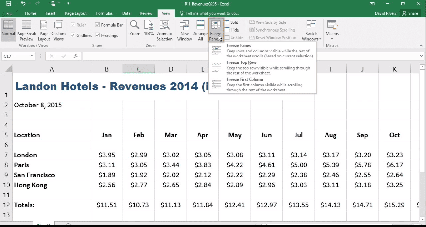
How to Freeze Cells in Excel So Rows and Columns Stay Visible

Image that shows how to freeze cells in Excel.

Have you ever worked in an unorganized spreadsheet? We have to admit, there is nothing more frustrating. When you scrolled down the endless rows, chances are, you couldn’t see your headers anymore. How are you supposed to keep track of where you are plotting data? This is where knowing how to freeze cells in Excel comes in handy.

If you have spent time working in a large worksheet, you may have wondered if there is a way to keep your rows and columns visible. This way, you can keep specific information visible when scrolling down or across. It is time-consuming and cumbersome to navigate back and forth to compare the top of your worksheet to the bottom. Luckily, Excel has a few built-in features to maximize your workflow efficiency.

Sometimes you may want to keep specific information visible while scrolling through your spreadsheet. In this case, Excel’s “Freeze Panes” feature is useful. In this article, we will show you all the ways to freeze the cells and how to do so where rows and columns stay visible. Here are a few tips to keep in mind when learning how to freeze cells in Excel.

  • Excel can only freeze panes from the top down and left to right.
  • Panes cannot be frozen while in “Edit” mode.
  • Frozen Panes can easily be unfrozen.

When and Why You Should Learn How to Freeze Cells in Excel

As mentioned earlier, unnecessary scrolling in Excel is a waste of time. It takes longer than you might think just to scroll up and peek at your category labels. It’s essential to minimize wasted time so you can get your work done efficiently.

In many cases, your spreadsheet will fill up more than what is visible on your screen. Any given worksheet contains a maximum of 1,048,576 rows and 16,384 columns. Thankfully, most spreadsheets will not meet their maximum capacity.

If you are working with several categories, it is helpful to keep your headers on screen at all times. Hence the need to learn how to freeze cells in Excel.

How to Freeze Cells in Excel

Although it’s not obvious at first glance, learning how to freeze cells in Excel is a simple process. While this feature is quite useful, it does have its limitations and can be a bit finicky at times. Below you will find out how to freeze panes and some common pitfalls to avoid.

Freezing the Top Row

Let’s start with freezing the top row of a worksheet. Freezing the top row is probably the most common use of the “Freeze Panes” feature. Freezing the top row of a spreadsheet allows you to keep your headings in place so that you can see them while scrolling.

To begin, select the “View” tab on the Ribbon at the top of your page. In this tab, you can check to ensure that your worksheet is in the “Normal” view and also select your desired “Freeze Panes” options. The “Freeze Panes” tool will not be available if your worksheet is not in “Normal” mode.

With your worksheet in “Normal” view, click the drop-down arrow on the “Freeze Panes” icon. You can then select “Freeze Top Row” from here. The top visible row of your worksheet will now be locked in place at the top of your spreadsheet.

Please note that the “Freeze Top Row” option freezes the top visible row of the current spreadsheet. If your worksheet was not scrolled all the way up, you might have frozen your spreadsheet farther down from the actual top. This feature is useful if you want to compare a row in the middle of your spreadsheet to one at the bottom.

If you freeze a “top” row that is not the first row of the worksheet, Excel will hide all rows above the frozen row until you unfreeze your “top” row.

Freezing the Leftmost Column

Let’s say that you’re working in a large worksheet with a list of dates on the leftmost side of the page and multiple categories across the sheet. If you want to keep your dates visible while exploring all of your categories, you will need to freeze the first column of your spreadsheet.

Freezing the first column of your worksheet is precisely like freezing the top row. The only difference is that between the “Freeze Panes” drop-down menu you will select “Freeze First Column.”

Keep in mind Excel defines the “first” column as the leftmost visible column on the screen. If you want that to be your very first column, you must have your worksheet scrolled entirely to the left when selecting this option. Otherwise, you can use this feature to freeze a column from the middle of your spreadsheet to compare it to the right side.

Just like when freezing the “top” row of a worksheet, freezing a column from the middle of the spreadsheet will hide all of the columns to the left until you unfreeze your “first” column.

More Options for How to Freeze Cells in Excel

It is possible to freeze more than one row or column at the same time. Additionally, you can freeze both rows and columns simultaneously. These features can be useful if you need to compare more than one row or column to other rows or columns that are too far separated to see.

To freeze more than one row, select the row below the last row you want to freeze. Navigate to the “Freeze Panes” drop-down menu and select “Freeze Panes.” Excel will freeze all of the rows above your selected row.

Freezing multiple columns is very similar. Highlight the column to the right of the last column you want to freeze. Navigate to and select the “Freeze Panes” option. This freezes all the columns to the left of your selected row.

To freeze rows and columns at the same time, select the cell that is under the last row you want to freeze and to the right of the last column you want to freeze. Navigate to the “Freeze Panes” option and select it by clicking.

To unfreeze rows or columns, select “Unfreeze Panes” from the “Freeze Panes” drop-down menu.

Despite its limited functionality, the “Freeze Panes” feature is handy for working with large worksheets. Knowing how to freeze cells in Excel may take a little practice to master. Have patience while learning the valuable skill and you will reap the benefits of a much more efficient workflow. Excel is a robust program with solutions for nearly every problem you will encounter.

Here’s a Shortcut to Freeze Cells in Excel

Did you know that there are handy keyboard shortcuts for Microsoft Excel programs? Using these shortcuts not only saves you work time but also from pesky, repeated actions. The main reason why people use shortcuts for Excel is that they do not have to take their hands off the keyboard to use a computer mouse and visually search for both menus and buttons. For example, let’s say that you want to add a new workbook. Without using a keyboard shortcut, you would have to click the “office button,” select “new,” and then double click the “blank workbook” icon. Did you know that you can just click Cntrl + N (The control key clicked with the button for n)? The following abbreviations will make your work life a whole lot easier. 

  • Shift + Space: This shortcut will select a row. 
  • Ctrl + C: Use this shortcut to perform the copy action.
  • Shift + Ctrl + Arrow Down: With this combination, you can select all the way down to the bottom of a region within Excel. 

How to Freeze Cells: Final Review

That is it. You see, learning how to freeze cells in Excel is not as daunting as it may have seemed. With these tools and handy shortcuts under your belt, you are well on your way to workplace efficiency. 

how to use goal seek in excel

How to Use Goal Seek in Excel

Excel has proven itself to be very useful in various situations over and over again. The list of Excel’s benefits seems to be never-ending.

It even has a tool for answering questions and forecasting information. The Goal Seek function in Excel is a great tool for those asking “What if” type questions.

Use this guide to learn how to use goal seek in excel as well as how to put it into action.

Why Use Goal Seek?

why_use_goal_seek_


The Goal Seek feature in Excel is basically used to create formulas. It provides information on cause and effect situations.

It determines what specific data will impact another set of data. This feature comes in handy in lots of scenarios.

In financial and sales situations, it can be used to determine what must be accomplished in order to reach a certain monetary goal.

It can also be used to calculate how many votes a candidate needs to win an election.

Once you have your Goal Seek formula in place, you can change any part of it to see how the formula as a whole change.

For example, a computer sales company has a profit goal of $3 million for the year.

Each of their computer systems cost $200, while additional accessories like keyboards cost $50 extra.

This company could use how to use goal seek in excel to determine how many of each product they’ll need to sell to reach their goal.

Here’s How To Use Goal Seek In Excel

To use Goal Seek, you will have to open a new sheet and enter the current information you have.

To make learning Goal Seek a little easier, we are going to use a simpler example.

Sample Scenario

how to use goal seek in excel

How To Start

To start, enter your information and functions into a spreadsheet in an organized table.

For our data, we’ll have the headings Playground, Movie, and Total in the first column.

Across the top, we’ll have the headings Votes and %. We have set up our table to calculate percentages base on the votes.

The goal will be to determine how many votes will it take to choose the Playground option.

Next Move

The next thing we need to do is select the cell we want to change. We want to make the Playground vote equal 66%, or 2/3, so we will select that cell.

Under the Data tab, locate the “What If Analysis” button. Click it to reveal the drop-down menu.

On this menu, you will see “Goal Seek.” Select this option, and a dialogue box will appear.

The first option you will see will ask you to set your cell. In our case, the percentage of Playground votes cell is D2, so we will enter that into the box.

Next, you will see “To value.” This is where you enter the desired goal. Our goal is 66%, so we will enter that into this box.

Final Steps

Finally, the last box will say “By changing cell.” This will be whichever cell you want to change in order to get your result.

We want to know how many votes will get us to 66%, so we want to change the number of playground votes. In our case, that is cell C2.

After you input all of your information, hit OK. Your information on your table will change to accommodate the goal number you have set.

In our case, we change the playground percentage to 66% based on the number of votes it needs.

When we hit OK, the numbers on our chart revealed that 24 out of the class’s 37 students would have to vote for the playground.

That is for them to reach 66% and establish a fair vote.

The Goal Seek function also shows us that for this to be true, 13 students will have voted for the movie.

Conclusion


how to use goal seek in excel

The Goal Seek function can be a very useful tool when trying to forecast sales, finances, votes, etc.

Numbers can be tricky to determine, and in important situations, it can be crucial to making decisions based off of accurate information.

The Goal Seek serves to perform exactly that.

Upon first use, the function can prove to be a little tricky. An important thing to remember is to make sure all of the functions in your table make sense.

The Goal Seek feature will not work properly if your functions don’t add up.

You may also get some funky numbers that don’t make sense if your functions don’t make sense.

It is a good idea to practice using this method a few times before you start using it for important projects.

Once you have the feature mastered, Goal Seek is an excellent tool for both professional and educational use.

Read through this guide on how to use goal seek in excel and follow the steps a few times to really nail down the skill.

This may come as a surprise to how useful it becomes. As a matter of fact, your business or job will be a lot easier.

Soon you’ll be forecasting information for all sorts of projects!

How to add cells in Excel (screen shots of cell data added up via the SUM formula).

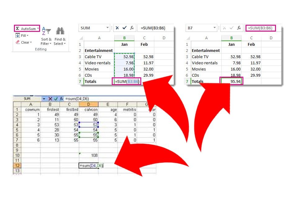
How to Add Cells in Excel to Sum Up Totals Automatically

Excel’s great for displaying data and even better at crunching numbers. Here’s how to add cells in Excel to sum up totals automatically… Even when you change the numbers.

A great feature that Excel has to offer is its use of formulas. Since Excel is often used to organize numerical data for a variety of operations, it can be beneficial to have an ‘addition’ function. In this guide, we are going to discuss the various ways we can add cells in Excel.

Why is the Addition Function Useful When You Need to Add Cells in Excel?

As we already know, in Excel Worksheets we can add columns. However, sometimes it is necessary to add cells that are not in columns or are not even next to each other.

For example, let’s say you are performing a survey to present data. You are interviewing random students to find out the most popular subjects taken in school. Your poll is anonymous, allows students to select only one option, and is organized by gender and grade levels Freshman, Sophomore, Junior, and Senior. The survey offers several subjects.

This survey is set up to give you a wide range of information and a variety of totals for you to examine. You could add these totals yourself, or you could use the many ways to add these numbers to Excel.

How to Add Cells in Excel: Method 1 (via Individual Table Cells)

In addition to adding columns in Excel, you can also add horizontally in rows. Let’s say you want to know how many senior males were surveyed. You can do this by adding up all the numbers in the Senior Male row. Let’s say the Senior Males row is row two in columns B2 through H2. One way to add your numbers is to select cell I2 and type the equals (=) sign, followed by the numbers in each cell in that row. For example, it may look something like this:

=5+6+2+7+0+9+1

Then, hit the enter button and you will get your total. While this method works, you will not be able to change the numbers in your cells without also changing your formula.

Because of this problem, it is better to enter the cells than the information within them. Rather than the above example, your formula will look similar to this:

=B2+C2+D2+E2+F2+G2+H2

When you hit Enter after typing this, you will still get your total. However, this time, you will be able to change the information in these cells, and the change will automatically affect the total.

How to Add Cells in Excel: Method 2 (Sum Function)

There is another method to adding rows. In this method, select your total cell. In our case, it has been cell I2. Type the equal (=) sign. Next, click the first cell in your row, or B2. This cell will become highlighted and appear next to the equal (=) sign. Then, type the plus (+) sign and click the next cells in the row. Continue this until you have clicked every cell in the row. Hit Enter to view your total.

Finally, rows can be added in the same SUM Function that we learned with columns. In your total cell, type =SUM. Then, type or click your beginning cell. Type the colon (:) mark and then type or click on the last cell in your row. It will look something like this:

=SUM(B2:H2)

Hit Enter when you have completed this function, and your total will show up. In this function, you can also change the values in each cell, and the changes will be reflected in the sum.

How to Add Cells in Excel: Method 3 (Adding Up Individual Cells In Different Rows and Columns)

The great thing about the addition function in Excel is that you not only get to add rows or columns. You can also add whatever cells you want to. Let’s stay with our survey example. Perhaps you want to examine precisely how many girls prefer math and science. Excel allows you to do this.

Label your first cell to maintain organization in your document. Click the cell next to it to begin your equation. Type the equal (=) sign, followed by all the cells you would like to add together. For example, your equation may look like this:

=C3+C5+C7+C9+D3+D5+D7+D9

Hit the Enter button when you are finished to get your total.

Of course, as we have already learned, it can be a bit tedious and take a while to type all of that. The alternate method would be to click instead of type. In your total cell, type the equal (=) sign. Then, click your first cell. Type the plus (+) sign and click your next cell. Continue this process until you have clicked all the cells you want to add. When you have selected all your cells, hit Enter to get your total.

Using this method allows you to select any cell that contains a numerical value. The values do not have to be in the same row or column or be next to each other. This method also allows you to change information in cells used in your formula. The modified data will automatically update the total to reflect the new numbers.

Conclusion

It was certainly good news to hear that we can add columns of information within our Excel Worksheets. It made life a lot easier and minimized the work we had to do.

Now, we see that we can also add rows as well as individual cells. This guide has expanded what we can do with the addition function. This function could be vital information when it comes to surveys, projects, and organizing business or personal information.

Follow this step by step guide to add cells in Excel using the addition function to its fullest, incorporating rows and cells into your skill set.

The 24-Hour Rule

A long time ago I was doing some reading on how you write and publish blog posts. One suggestion that helps me is the 24-hour rule. And that is to finish your post and then wait 24 hours before reading it one-last-time. After all, a blog post is going to be public, out there on the internet with your name on it, for a very long time.

The problem with this 24-hour rule is that I usually find one or more things that need to be changed. And then I have to wait another 24-hours.

When you are on a deadline, like, for instance, having a self-imposed quota of 2 or 3 blog posts a week, the 24-hour rule is inconvenient. It drives you to compromise on the level of quality.

By that I mean that there is a hierarchy of quality levels starting with spelling and grammar and ending with saying what you intended in the most concise, articulate manner possible. A deadline drives you to ensure the spelling and grammar are correct and then you compromise on just how well you get your point across.

Tech Man

For me the deadline and quality levels force a certain tension, all of which drove me to abandon my blogging of all things Excel. Yet since a deadline and quality levels are self-imposed, they are also controllable.

I’ve decided to stick with the 24-hour rule and forget about the deadline, or any deadline for that matter. Consequently my blogging will continue, at my own pace.

Right now I’m working on a post about the Excel iPad app.

So the 24-hour rule stays and the journey continues.

Where is Control+Home for Excel on a Mac

I wrote a post stating that I could not find the Windows Ctrl+Home keyboard shortcut equivalent on a Mac. Well I’m here to tell you that I found the keyboard shortcut combination that does the same thing on a Mac. The Excel Gods are with me. Hallelujah!

Finding My Way Home

The key to finding this elusive keyboard shortcut is in the Keyboard Viewer. On your Mac select the Apple icon () and click System Preferences… Select Keyboard, and then make sure to click the Keyboard tab. Check the box for: Show Keyboard & Character Viewers in menu bar.

Excel home key on mac

Click the Keyboard Viewer icon Keyboard Viewer Iconin your Mac menu bar and a nice replica of your Mac keyboard will appear.

Keyboard Viewer Mac

You will notice that this viewer reflects the keys you tap on your keyboard. The screen shot above shows the Command and Shift keys are depressed. The Keyboard Viewer will also show different symbols when you press various keys, like fn, Control, Option, Command, etc.

This is where I noticed something interesting. While depressing the fn key, the left arrow button changes its angle to point up about 30 degrees. Knowing that allowed me to do a little testing in Microsoft Excel 2011 for the Mac.

Excel Control+Home Key on Mac

What I found is that the Windows Control+Home keyboard combination can be replicated on a Mac by either of the following keyboard shortcut combinations. This is the home key on Mac:

fn+Command+Left Arrow

fn+Control+Left Arrow

Another mystery solved.

Keyboard Shortcuts

Another aid in finding keyboard shortcuts comes in the form of an overlay for your Mac keyboard. The kind folks over at Excel Skin™ gave me an overlay that slips over the Mac keyboard and shows, via color coding, a wide array of shortcuts that work in Excel for Mac. Here is why you might want an excel skin.

Copy Symbol Image

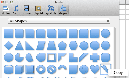
Add Macro Button to the Toolbar in Excel 2011

You can add an icon to the toolbar in Excel 2011 for your Personal Workbook Macro. In an earlier post I created a short macro to imitate the Control+Home keyboard shortcut in Excel for Windows. You can add an icon to the toolbar to run that, or any other macro with a few quick steps.

  • Right click on the toolbar and select Customize Toolbars and Menus… then
  • Click the Commands tab, then
  • Scroll down and select Macros from the Categories pane, and
  • Drag the Custom Button with a smiley face to the toolbar, then
  • Click OK to get rid of the dialog box.

Next you:

  • Right click on the smiley face, select Assign Macro… and
  • Pick the macro you created (in your personal macro workbook), then
  • Click OK.
  • Change the Smiley Face Image

    If you don’t like the smiley face icon staring back at you want to change it (like I did) that’s easily done as well.

  • Right click on the Custom Button icon and select Properties… then
  • Type a name in the Name: box, then
  • Click the drop-down arrow beside the smiley face and select from the icon list, then
  • Click OK.
  • Use a Custom Image for the Toolbar Button

    The icon list is rather short and pathetic, but you need not restrict your choices as Excel allows you to copy and paste an image into the button face. Here is how I changed my smiley face image.

  • Choose Insert > Symbol
  • Click Shapes (at the top of the dialog box)
  • Right click on your favorite shape and click Copy, then

  • Copy Symbol Image

  • Close the Media dialog box, and
  • Right click on the smiley face toolbar icon, then
  • Click Properties…
  • Click the drop-down beside the image, and
  • Click the option Paste Button Image, then
  • Click OK.
  • Move Your New Macro Button

    In case you didn’t get your button located in the right place on your toolbar when we first started this exercise, the button is easily moved.

  • Right click on the Toolbar and select Customize Toolbars and Menus…
  • Drag your icon to a position of your choice, then
  • Click OK.
  • Personal Macro Workbook GoHome Code

    Control + Home in Excel for Mac

    One of my all-time favorite keyboard shortcuts in Excel is CTRL+Home, but on a Mac there is no Home button. Hence a constant source of frustration these last two years.

    I finally decided to do something about that and recently figured out a solution using VBA and the Personal Macro Workbook. But before I go straight to the answer, let me tell you how I got there.

    My Journey

    I knew that VBA was going to enter into the equation, so I started to record a macro on a Windows PC while using the Control+Home keyboard shortcut. What I found out is that Excel does not record that keyboard shortcut. Nothing, nada, zip.

    I then noticed that Control+Home acted differently, depending if the sheet panes were frozen or not. When sheet panes are not frozen, the Control+Home shortcut took me to cell A1. When the sheet panes are frozen, then the upper left corner cell of the window was selected.

    To make a long story short, I found out that the active window’s scroll row and column were being selected when the CTRL+Home shortcut is executed in Excel for Windows.

    The Control+Home Macro

    I also knew that if a Chart sheet were selected the macro would fail, so I crafted the following macro to mimic the CTRL+Home shortcut on a Mac. (Works on a Windows PC too.)


    Sub GoHome()
    '''''''''''''''''''''''''''''''''''''''''''''''''''''
    ' Make sure the active sheet is a worksheet,
    ' then locate the active window's scroll row and
    ' column, and activate that cell.
    '''''''''''''''''''''''''''''''''''''''''''''''''''''
    Dim lngRow As Long
    Dim lngCol As Long

    If ActiveSheet.Type = xlWorksheet Then
    lngRow = ActiveWindow.ScrollRow
    lngCol = ActiveWindow.ScrollColumn
    Cells(lngRow, lngCol).Activate
    End If
    End Sub

    The next thing I did was create a shortcut for the macro, but realized that the macro would only work with the current workbook. Rats!

    I wanted the macro work automatically on every Excel file so I chose to store this macro in the Personal Macro Workbook, which solved the problem.

    However the shortcut key combination I assigned did not work in Excel for Mac. There was a conflict. It seems that COMMAND+OPTION+H is a reserved keyboard shortcut for the Mac. I found out this shortcut hides all windows except the one that is active.

    How I Created the Control+Home Keyboard Shortcut on my Mac

    Here are the steps I took, with a few false starts along the way.

  • Open Excel 2011 and choose Tools > Macro > Record New Macro…
  • Type a name for the macro. I used GoHome.
  • Enter a Shortcut key. (I used h, which didn’t work so I changed to g as you’ll see below.)
  • Where you see Store macro in: click the drop-down and select Personal Macro Workbook.
  • Click OK.
  • Record Macro Dialog Box

    I got a warning that the keyboard shortcut Option+Command+h was reserved.

    Reserved Shortcut

    So I chose g instead and clicked OK.

  • Next choose Tools > Macros > Stop Recording. This will effectively end the macro recording without recording anything.
  • Choose Tools > Macro > Macros…
  • Macro Dialog Box

  • Click the Step Into button on the Macro dialog box, which will take you directly inside the macro in the VBA Editor. (Note: While this takes you directly to the macro, it also starts the macro running inside the VBA Editor.)
  • Reset the Macro

  • Click the square Reset button to stop the macro program execution. (Note: If you know how to navigate the VBA editor, you can skip this last step and choose Tools > Macro > Visual Basic Editor and then locate the macro.
  • Select the entire GoHome code from this article. Or click this link and copy from a new window.
  • Copy the text,
  • Switch back to the Excel VBA editor,
  • Select the entire GoHome subroutine, and
  • Paste the code.
  • Personal Macro Workbook GoHome Code

  • Close the VBA editor by choosing Excel > Close and Return to Microsoft Excel.
  • Close VBA Editor

    Now here is the important part so pay attention. You have to save changes to the Personal Macro Workbook. You will be asked to do this when you Quit Excel.

  • Choose Excel > Quit Excel and the following dialog box will appear.
  • Save Personal Macro Workbook Changes

  • Click the Save button when asked, “Do you want to save the changes you made to the Personal Macro Workbook?”
  • Run the GoHome Macro

    Now lets check it out. Open Excel 2011 and select any cell that is not A1, then use the shortcut (mine was Command+Option+g) and watch the active cell change to cell A1.

    If your shortcut doesn’t work you can set it now. Choose Tools > Macro > Macros… and select the GoHome macro, then click Options. Type in a shortcut key and click OK.

    Now choose any cell in the top left quadrant of the current window, like C5. Choose Window > Freeze Panes. Next select any cell except C5 and run the shortcut combination for the macro, and watch the curser jump to cell C5.

    The Personal Macro Workbook will load each time you open Microsoft Excel so it’s always in the background, and you don’t get that annoying “enable macro” pop-up screen.

    Related Posts Plugin for WordPress, Blogger...