Those wondering how to create a drop down list in Excel will be relieved to know that it is easier than it sounds. As you may already know, drop down lists make data entry a breeze. For example, if you have ever used such a menu for surveys, polls, and web forms, you know how convenient they are. As tech nerds, we’re happy that such an option exists within an Excel spreadsheet.
Adding a drop-down list to a cell or range using Data Validation is a simple matter. Data Validation is used to define restrictions on what data can or should be entered into a cell. Here we’ll use a List to restrict what values can be entered into a cell. This article walks you through a step-by-step guide of how to create a drop down list in Excel.
How to Create a Drop Down List in Excel for a Cell or Range
Select the cell or range you want to use for a drop-down list, then
Choose Data Validation from the Data Tools group on the Data tab
Select the Settings tab
In the Allow box, select List
Click the Source box
Type in a list of values separated by a comma
Make sure the In-cell dropdown box is checked
Click OK
The list I created was for cell A1, which is shown below.
Excel 2010 Drop Down List
List Data Sources
Manually entering the source data for the Excel 2010 drop down list is probably the least desirable method. A better way is to put the list in a range, then refer to the range.
The same list data was put into the range J1: J6, then I changed the source reference to these cells. This is a better method than manually entering the values, but older versions of Excel require the list to be on the same worksheet. One way around this and a better solution is to give the List range a Name.
You can give the List range a Name then use it for the Source. For example, I selected the range J1: J6 then typed TheNames into the Name box, thereby creating a Named Range. On the Data Validation dialog box, I typed in =TheNames into the Source box.
Change the Reference to the Named Range
Now let’s assume that we have to add a couple more names to the list. Instead of changing every cell that references this Data Validation list, we just change the reference to the Named Range. (Choose Formulas > Name Manager, select the Named Range, change the reference in the Refers to box, then click the green arrow to make the change and click Close.)
But if the list will grow over time, changing the reference should be done automatically with a dynamic Named Range formula. We’ll do this by using the OFFSET formula.
Choose Formulas > Name Manager
Select New
Type a Name in the Name box (I’ll use myNamesList)
In the Refers to box type =OFFSET(Sheet1!$J$1,0,0,COUNTA(Sheet1!$J:$J),1)
Click OK
Now select the cell or range with Data Validation and,
Choose Data > Data Validation
Select the Settings tab
In the Source box type in =myNamesList (or the Name you created)
Click OK
This Named Range formula is dynamic, which means the source list will expand when names are added to the list. If the list contains more than 8 values the drop-down list will have a scroll bar.
Excel – Pick from Drop Down List
Bonus Tips
One of the things we love the most about creating a drop down list in Excel is that the program reminds you to save your work before you click out. However, the program will not remind you to create a backup. If you do not have an automated backup system in place, we highly recommend implementing one. For example, you can download and save a copy locally to your desktop and USB drive. If you are using a thumb drive, store the saved copy offsite. Does this sound like overkill? Maybe. But you will not think so if you lose your first copy and then find yourself in need of it.
How to use a drop down list in Google sheets.
If you are not close to a device with Excel, you might have to use spreadsheets. Things in spreadsheets are simple. All you have to do in order to create a drop down list is to select the columns you need and afterward to go to Data. Then you will have to select data validation.
In spreadsheets, data validation gives you the following criteria: List from a range, List of items, Number, Text, Date, Custom Formula, and Checkbox. Also, you can allow someone to type invalid data or to reject it by default.
You can also create a Yes/No Drop down list, by using the criteria “List of items” and by typing in the box yes and no separated by a comma. The last step is to choose the option “On invalid data reject input”.
Another thing you can do with Google sheets is to search for the items in your list by just using a few letters from the word. This comes in handy when you have a long list of names or terms and you want to find a specified one or a group of them.
How to Create a Drop Down List in Excel: Final Thoughts.
Now that you know how to create and use a drop down list in Excel and Google Sheets, you can have fun and do some easy exercises. Try to organize what each member of your family wants to eat for a week or use a spreadsheet as a grocery list.
With Google Sheets, you can also do some real time checkups with your friends or family members. Just share the spreadsheet with them and let them come up with the needed items for the events you are attending together.
That’s it. We hope you enjoyed reading our article on how to create a drop down list in Excel with data validation. It’s not as hard as you might have thought. Hopefully, you can now create a drop-down list that will meet your needs. Use as many drop lists as you need, now that you know how to make them it will only take you from a few seconds to some minutes. Anyways, Happy organizing!
Recently I was asked how to subtract time in Excel (time difference) or how to calculate the number of hours between two points in time on different days. Since this was in a reader comment, I gave a brief answer that requires a fuller account here.
Dates and Times are all part of the master plan in Excel. Once you “get” the fundamentals, the rest is just icing on the cake.
A Date value in Excel looks like this: 40519
A Time value in Excel looks like this: 0.58333
Cell formatting changes how you see these numbers.
The Date: 7 Dec, 2010
The Time: 2:00 PM
How to Calculate Time Between Dates in Excel or the Duration Between Two Dates
If you want to calculate time between dates in Excel or the duration between two dates, you need to understand what they mean first. When you type a Date into Excel, you may never see the underlying number, like 40519, but it’s there nonetheless. This is a date serial number and it makes Date calculations easy.
You might ask, “Why is this such a weird-looking number?”. Well, the Excel folks started a numbering system with Dates. In Excel for Windows they gave 1 Jan, 1900 the serial date number of 1, then continued numbering until this day and beyond. So serial number 40519 represents 7 Dec, 2010.
In Excel for Mac they started numbering Dates beginning with 2 Jan, 1904. (don’t ask) So the serial date 40519 represents 8 Dec, 2014 (Actually it’s known as the 1904 date system. To be clear, Macs can change Excel settings to use the 1900 date system).
How to Subtract Time in Excel (Time Difference)
When you type 2:00 PM into a cell in Excel the underlying value is a fraction, but Excel interprets this as a time serial number and formats the cell accordingly.
Try typing 0.25 into a blank cell, then change the cell formatting to a TIME format, and you’ll get something like 6:00 AM.
As an aside, you can calculate this fraction for any time value during the day by taking the total number of seconds that have passed from midnight until your time value and dividing by 86,400 seconds in a day.
Dates and Times Together
In Excel the unit of time is “the Day,” a key fact to know. You’ll notice that Dates are integers, and Time is a fractional number. You can add the two together to get a Date/Time format.
So adding a Date serial number, like 40518, to a Time serial number, like 0.25, gives us 40518.25. Formatting the cell holding this value using “d mmm, yyyy h:mm AM/PM” will show 6 Dec, 2010 6:00 AM.
You can also enter something like 7 Dec, 2010 2:00 PM into a cell and Excel will recognize this as a Date/Time format. However, if you change the cell formatting to General, the underlying number is 40519.05833.
So hopefully by now you can see that subtracting two Date/Time formatted numbers can be done mathematically. Subtracting 6 Dec, 2010 6:00 AM from 7 Dec, 2010 2:00 PM is done by Excel “underneath the hood” as 40519.05833 – 40518.25 and the result is 1.3333.
Calculating Hours Between Two Dates in Excel
If we recall that the unit of time is “the Day,” this value represents 1-1/3 days of time. Since there are 24 hours in a day, converting to hours is a simple multiplication 24 * 1.3333 = or 32 hours. (24 * 4/3 to be more precise)
Time Between Two Times / Dates
Finding the number of hours or the time between two times/dates is simple, just subtract the start date/time from the end date/time and multiply the result by 24 hours.
If you want to enter the dates and times separately (which is loads easier than typing in a date/time in one cell) then add the date/times together.
Here’s a look at a typical worksheet designed to calculate the hours between two dates.
As you can see, the formula for Hours, in cell F2, shows in the formula bar. And row 3 contains General formatting so you can view the date/time serial numbers for row 2.
Change the formatting for cells B2:E2 to match what you normally use for Date and Time data entry.
The NETWORKDAYS Function
People also asked how to calculate the time between days but without taking into account weekends or specified holidays. The NETWORKDAYS function will help you to calculate the time period by excluding weekdays and specified holidays.
The formula looks like this: =NETWORKDAYS(start_date, end_date, [holidays])
Like in the previous case the start_date and end_date are required arguments, yet the argument [holidays] is optional. You can use this argument to specify which days should be excluded.
This time I used two random dates which contained two weekends and I added two desired dates under the holidays argument just to show you how it works.
If you need to add some weekends you will have to add one more argument (weekends) and use =NETWORKDAYS.INTL(start_date, end_date, [weekend], [holidays])
After you calculated the days by using the NETWORKDAYS formula, to calculate the hours you can simply multiply the given number with the number of hours you need for as long as they stay the same. Also, do not work harder by looking for complicated formulas to calculate simple things.
What else you should know:
If the start date is later than the end date the formula will generate a negative number.
The NETWORKDAYS formula will also include the start and the ending dates in the calculations, due to this if you have the same date the value returned will be 1.
If you want to find more formulas regarding the date and time feel free to check the following list of functions.
I hope this article helps you to better understand how to calculate hours between two dates in Excel. You can exercise what you learned today by calculating the time left until your next birthday, to do this you can also use the =Today function or the =Now function.
If you found this article helpful, please feel free to check our other articles about tips and tricks in Excel. We also have a dedicated section for details and formulas about dates and times in Excel.
In this article, I will show you how to remove duplicates in Excel. While having duplicate data can be useful sometimes, it can also make it more difficult to understand your data. I’ll use conditional formatting to find and highlight duplicate portions of data within Microsoft Excel. Review your duplicate content and decide if you want to remove them.
Remember that when you delete duplicate values, the duplicate data is permanently deleted from your records. Before you go forward with deleting the duplicate content, I highly recommend that you copy the original data over to another worksheet. This ensures that you will not accidentally lose any of your vital information and hard work.
I use an iPhone app to record my food intake and exercise output every day, and also record my weight, albeit infrequently. All of this data is synced to a database in the cloud. The database automatically enters my weight each day, even though I don’t, by using the last known data point. All of this data can be downloaded in a CSV file, opened with Excel, and saved as a workbook file.
Charting my weight from this data is a simple matter, but Excel doesn’t need all of the extra data points. Consequently, I have reason to use the Remove Duplicates feature that was introduced in Excel 2007.
Using Dates with the Remove Duplicates Feature
I have two columns of data with Date in column A and Weight in column B. I want to remove all duplicate Weights but have to be careful because it makes a difference how the dates are sorted.
The file downloaded from the database was sorted in descending order by Date. When using Remove Duplicates I got a different result when the Dates were sorted in ascending order. In each case, the same number of unique Weight values were found but associated with different Dates.
How to Delete Duplicates in Excel
Understand how to delete duplicates in Excel: Apparently, the Remove Duplicates works from the top down so sorting dates in ascending order make sense. Keep that in mind when Date values are part of your data set.
Here is an example of the raw data, on the left, and the results from using Remove Duplicates when the data was sorted in descending versus ascending order.
Steps to Removing Duplicate Data in Excel
Select the data range or make sure the active cell is inside the data range you want to manipulate. Excel is smart enough to pick out the region of data and figure out if there are column headers.
First thing, make sure the data is sorted. I selected cell B2 and sorted the range in ascending order so the first unique Weight value would correspond to the First Date, and not the last.
Select Data tab » Remove Duplicates, which will bring up a dialog box.
Select the column(s) that have duplicate data
Check an see if the My data has headers box is checked (assuming you have column headers)
Click OK and you will eliminate duplicates in Excel
A popup box will confirm the number of duplicate and unique values
If you’re not satisfied with the result, use the keyboard shortcut Ctrl+Z to undo the Remove Duplicates action.
One of Excel’s most important features is the ability it gives users to quickly and easily sort through data. With this said, learning how to alphabetize in Excel is critical. If you are not familiar with this skill, don’t worry too much. We will go over alphabetizing lists of strings, ordering numerical values, standard alphabetization, reverse alphabetization, and more. Using Excel we can properly organize data for our businesses or personal finances. Learn how to alphabetize in excel so it is easy to read and refer back to whenever necessary.
What is Excel?
If you are a complete newcomer, you can still walk away from reading this article and learn how to navigate Excel. Let’s start with the basics. Before you learn how to alphabetize in Excel, we need to address the question ‘what is Excel?’ The answer is simple.
Microsoft Excel is a software application included within Microsoft Office Suite. You will use this tool to create spreadsheets (aka documents laid out in rows and columns). Due to the program’s versatility, it has become one of the world’s leading platforms in business since its initial launch in 1985.
What is an Excel Spreadsheet?
The next question you should be asking is ‘what is a spreadsheet?’ In short, spreadsheets organize data into easy ways to read and manipulate (rows and columns). An Excel spreadsheet is composed of columns (vertical boxes labeled ‘A, B, C, D…’ at the top of the screen) and rows (horizontal boxes labeled ‘1, 2, 3, …)’) at the left side of the screen. The intersection of each column and row holds cells where a user can enter either numbers or text. When one refers to the address of a cell, they mean the letter of the cell’s column combined with the row (e.g. A4).
How To Alphabetize In Excel
The main reason people use Excel is to organize data into an easy to read list. You want to be able to refer back to information from years ago, and quickly find something you need.
Excel is so useful because it gives you the ability to do just that. You can organize information alphabetically from A-Z or Z-A. This method allows you to create highly functioning spreadsheets that will keep all your data in order.
We’re going to break down:
How to alphabetize in Excel
Organizing columns that contain multiple strings of information
How to sort spreadsheets that have a combination of letters and numbers
Let’s dive right in!
The Reasons for Alphabetizing
For demonstration purposes, let’s say you are the owner of a sporting goods wholesaler and this is your spreadsheet for the month. If you look at the picture below, there is no structure to the data.
If you had a list built this way for ten years and you needed to look back during an audit. Then it would be incredibly difficult and time-consuming to find the information you need.
If we alphabetize the data, we could:
Scan through to find the name of a customer or product
Choose a specific department to document revenue
Find sales information on a particular product
Keep data organized for accounting and tax purposes
Additionally, if you have employees, having organized spreadsheets is even more critical. If you can’t make sense of your data, your employees will never understand it.
Basic Alphabetization
There are a variety of ways to organize information in Excel. However, we will start with the simplest method and work our way up.
Firstly, highlight the columns or rows you would like to sort by clicking and dragging your mouse across the cells.
Click the Sort & Filter button on the top right of your dashboard, and you will be able to sort Ascending from A-Z, or descending from Z-A.
Accordingly, doing this will organize the columns you have selected alphabetically. As you see above, I arranged the Customer column from A-Z.
One thing to remember:
It’s important to make sure you do not have empty spaces or special characters in front of your data.
Advanced Alphabetization
Alphabetizing in Excel is easy when you are sorting one column. Things get interesting when you have multiple columns, and you need to keep them in order as well.
Let’s say you want to organize alphabetically by the customer. But you also want to keep those customers in groups based on departments they purchase from. You can do that using Excel’s custom sort feature.
Firstly, select all your data by dragging your mouse over everything or clicking the arrow pointing diagonally towards your spreadsheet. Then make sure you highlight the entire spreadsheet – if you are missing cells you won’t have everything sorted.
Next, go back into the Sort & Filter drop-down box and select Custom Sort. Your screen may vary slightly depending on which version of Excel you are using.
In the box above, you will see that there are a few options for sorting your data. Under column, you can choose what header you are sorting. For this example, we will sort by “Product.”
The next option you see is “Sort On” – this is what your cell is based on. For example, we will always leave it as “values.” You can sort based on cell color, font color, and more.
Lastly, you can choose the order for which you are sorting. You can sort ascending from A-Z or descending from Z-A when learning how to alphabetize in Excel.
If we do this, we will have our product list sorted from A to Z similar to the first demonstration, but this time we are going to get more advanced and add another level to the sorting.
In the custom sort dialogue box, click add level, and you will see another row appear.
The second line is labeled “Then by” – this level of sorting will follow whatever is in the first line. Whatever column you include here will sort after your first line of data.
For our example, we will use Revenue as our column to sort after we have alphabetized our products.
We will leave “values” as what we are sorting based on and this time we are dealing with numbers instead of letters – we were given a different option for “order.” We want to sort our revenue from Largest to Smallest to find out what products are our best sellers.
Once you have everything set up and you’re ready to organize your data, press OK, and you now have a spreadsheet that is organized by product first and revenue second.
Looking at this organized spreadsheet, you can quickly identify what your best-selling product in the football department is footballs in packs of 5.
Alphabetizing in a Custom Order
Up until this point, we have been organizing data ascending or descending.
You are probably asking – How do I arrange chronologically by month?
If you organize months alphabetically, February will come first so that would not work. We are going to show you how to get even more technical and organize chronologically.
First, go back to Sort & Filter and open up Custom Sort.
We have added a column for the month now.
Under “order” in the custom sort box, you will choose “custom list,” and it will bring up this dialogue box:
Here you will manually enter the order you want the entries to appear. In this example, we want to order the data – January, February, and March. Click OK to confirm then hit OK again to sort.
Finally, you have a completed list that is organized by Product, Revenue, and Month.
Why Isn’t My Spreadsheet Sorting?
It could be the wrong selection. On the off chance that you chose the off-base lines and sections or not exactly the full cell extend that contains the data you need to sort, Microsoft Excel can’t organize your information the manner in which you need to see it. With a fractional scope of cells chose, just the determination sorts. With void cells chose, nothing occurs. To sort every one of your information without making a choice first, click in one cell inside your information extend. When you open the Sort discourse box, you can see a choice zone encase the information that Excel will arrange.
Effectively Sorted
Issuing a sort direction on an informational collection that you’ve effectively arranged, or that you entered utilizing prearranged information, creates no unmistakable outcomes. Excel reacted to the direction you mentioned, but since you effectively composed your data, you can’t sort similar information twice into a similar request. To re-try your sort and really make a redesigned outcome, you’ll have to adjust your sort parameters.
Off-base or Mixed Data Type
On the off chance that you key in a segment of dates into cells that you’ve set up in a blend of content and date designs, your information won’t sort effectively. By blending your cell groups, you’ve set up a line or segment that contains what could be compared to apples and oranges rather than only either. How you show your information additionally can impact how you translate the aftereffects of a sorting task. Dates that show with just their month and day indicating may sort in a startling request since they really originate from various years. When you see odd outcomes, for example, these, you may need to check your information and cell types.
Additional Considerations
Record or application debasement dependably can create unexpected outcomes even in routine programming activities, for example, a worksheet information sort. On the off chance that checking your information and your worksheet configuration doesn’t resolve your arranging issues, shut down Excel and restart your PC to check whether your outcomes change. You additionally can duplicate your worksheet substance, glue them into another Excel record and attempt your sort task there, viably precluding – or distinguishing – your document as the wellspring of your concern.
What is the Difference Between a Workbook, Worksheet, and a Spreadsheet on Excel?
When you open Microsoft Excel (a spreadsheet program), you’re opening an exercise manual. An exercise manual can contain at least one distinct worksheets that can be gotten to through the tabs at the base of the worksheet your at present survey. Often most confounding that a worksheet is synonymous with a spreadsheet. At the end of the day, a spreadsheet and worksheet mean something very similar. Be that as it may, a great many people just allude to the program like a spreadsheet program and the records it makes as spreadsheet documents.
Spreadsheet Programs
Today, Microsoft Excel is the most prevalent and generally utilized spreadsheet program, however, there are additionally numerous choices. Despite the fact that spreadsheets are regularly utilized with anything containing numbers, the employment of a spreadsheet is practically interminable. The following are some other prominent employments of spreadsheets.
Account
Spreadsheets are perfect for money related information, for example, your financial records data, spending plans, charges, exchanges, charging, solicitations, receipts, conjectures, and any installment framework.
Structures
Structure layouts can be made to deal with stock, assessments, execution audits, tests, time sheets, persistent data, and reviews.
School and Grades
Instructors can utilize spreadsheets to follow understudies, figure reviews, and recognize pertinent information, for example, high and low scores, missing tests, and understudies who are battling.
Records
Dealing with a rundown in a spreadsheet is an extraordinary case of information that does not contain numbers, yet at the same time can be utilized in a spreadsheet. Incredible instances of spreadsheet records incorporate phone, to-do, and basic food item records.
Sports
Spreadsheets can monitor your preferred player details or details in the general group. With the gathered information, you can likewise discover midpoints, high scores, and factual information. Spreadsheets can even be utilized to make competition sections.
What is a Functioning Worksheet?
A functioning worksheet is a worksheet that is as of now open. For instance, in the Excel picture over, the sheet tabs at the base of the window show “Sheet1,” “Sheet2,” and “Sheet3,” with Sheet1 being the dynamic worksheet. The dynamic tab ordinarily has a white foundation behind the tab name.
Why Not Use a Word Processor Instead of a Spreadsheet?
While the facts may prove that a portion of the things referenced above should be possible in a word processor, spreadsheets have a tremendous preferred position over word processors with regards to numbers. It is difficult to compute various numbers in a word processor and have the estimation of the computation quickly show up. Spreadsheets are likewise significantly more unique with the information and can hide, show, and sort data to make handling loads of data simpler.
How to Alphabetize in Excel: Final Review
Finally, Excel is an incredibly useful tool for business owners, entrepreneurs, and those who are financially savvy. This covers everything you will need to know about how to alphabetize in Excel. Follow this article step by step, and you will have no problem finding anything and everything you need to know for years to come! If you want to learn how to make a line graph, hiding columns or freezing rows in excel, then we have them for you too.
When working with Excel spreadsheets, it can be difficult to extract the information you need from large sets of data. Pivot Tables (pv table) offer a great way to quickly condense and analyze, and present your data, allowing you to make informed decisions in both your professional and personal life.
Pivot Tables allow you to effortlessly summarize large amounts of data into a simple format that’s easy to read and analyze. You can subtotal numeric data, sort information into subcategories, or create custom calculations and formulas to focus your results.
Here, we’re going to discuss everything that you need to know about a PV Table, including:
Why you should use Pivot Tables
How to create a Pivot Table
What you can do with Pivot Tables
What are Pivot Tables (AKA Pv Table)?
Pivot Tables, also known as Pv Tables, are an Excel tool that allows you to organize data in a way that’s easy to understand. You can use data from a spreadsheet or import a database table to access the information you need. Excel is able to connect to external sources such as SQL Server tables, Azure Marketplace, Office Data Connection (.odc) files, XML files, Access databases, and text files. Making a Pivot Table won’t alter your original data in any way, but instead will arrange it into a tabular format that makes sense and is easier to read than the original spreadsheet.
The Advantages of Using Pivot Tables
The main function of Pivot Tables is to help you organize large quantities of data in a way that’s quick to analyze. You can filter and sort groups into a table that’s more user-friendly than a raw data set or spreadsheet. Pv Tables also make it easy to expand or collapse rows and columns to narrow down your results, giving you a more detailed picture of important data while cutting out unnecessary background noise.
Not only do Pivot Tables make it easier for you to track data more effectively, but they also make it easier to present information. Whether you’re speaking to family members, co-workers, or supervisors, Pivot Tables give a clear and concise picture of your data that’s easy on the eyes.
If you’re not happy with the layout of your Pivot Table, Excel makes it easy to manipulate and reformat information. Not only can you sort, filter, and group data. But you can also add, rearrange, remove, or change the order of fields. You can also easily change the Pivot Table form, choosing between Compact, Outline, or Tabular.
Tables are in compact form by default, but this may not suit your needs if you want headings for Row fields. If this is the case, you can switch your Pivot Table to Tabular Form, which displays one column per field and provides space for field headers, or Outline Form, which displays subtotals at the top of every group.
Creating Recommended PV Table
Pivot Tables are easy to make with just a few clicks of a button. If you’re new to Excel or Pv Tables in general, you may want to start out using Recommended Pivot Tables. This feature automatically comes up with a layout to match your data set. If you aren’t pleased with the final result, you can always experiment by tweaking rows and columns. To create a Recommended Pivot Table:
Click on any cell in your original data set or table range.
Go to Insert > Tables > Recommended Pivot Table.
Excel analyzes your data and presents you with several options based on the categories it detects in your data.
Select whichever table looks like it will best suit your needs. And then hit OK to create a Pivot Table on a new Excel sheet.
The Recommended Pivot Table feature is a relatively new one, introduced in 2013. It’s only available for users that have the Office 2013 suite or above. If you have an earlier version of the software, you’ll have to create Pv Tables manually.
Manually Creating Pivot Tables
Creating a Pivot Table manually is just slightly more complex than making a Recommended Pivot Table. In addition, it gives you more control over your end results and only takes a few more steps. Here’s how you can manually create a Pivot Table to display your data:
Click on any cell in your original data set or table range.
Go to Insert > Tables > Pivot Table.
A box will pop up displaying the Create Pivot Table dialog. You can select and name a range of Excel cells, or import from an external data source. If you want to analyze multiple tables at once, check the “Add this data to the Data Model” box at the bottom of the popup screen.
On this screen, you can also choose whether you want your report to be opened in a new sheet or an existing worksheet. If you choose to place your table in a current worksheet, you need to select both the file and the cell where you want your Pivot Table to be stored.
Click OK, and you’ll see Excel create a blank Pivot Table and display the Pivot Table Fields list. Here, you’ll select the checkbox for any field you want to add to your Pivot Table.
Using Pivot Tables
Once you’ve finalized the formatting of your PV Table, you can take things one step further. You can turn it into a Pivot Chart.
This gives you an even more powerful way to display data. Especially if you’re planning on using it in a presentation. Pivot Charts add visualizations to data in the form of a graph or other chart type.
This makes it easy to summarize data and spot trends and patterns over time. Pivot Charts automatically update when you adjust your Pivot Table.
Conclusion
Excel is a powerful tool both at home and in the office, but datasets and spreadsheets can get confusing. Pivot Tables help you to make the most of your data. It allows you to eliminate unnecessary information and highlight what’s important to you or your business.
By using Pivot Tables, you can quickly come to conclusions and make informed decisions based on large caches of data. Pivot Tables also make it easy to wow bosses, coworkers, and investors during presentations.
Follow the steps laid out in this article. Spare yourself from a headache by effortlessly organizing and analyzing large data sets using Pivot Tables.
Whether you’re keeping on top of your home life or climbing the corporate ladder. Pivot Tables can come in handy when analyzing and presenting data.
I have a worksheet that tracks start and stop times for different events throughout the day, all during the week. Sometimes I have to pull out the Time of Day, irrespective of the Date, with the TIME function.
The TIME function has three arguments: Hour, Minute, Second. I could use =TIME(11,30,0) in a cell to get 11:30 AM, but I want to convert a Date-Time number so let’s look at an example.
In cell C2 I have the Date-Time value 10/8/12 6:28:30 PM.
In cell B2 I enter the formula =TIME(HOUR(C2),MINUTE(C2), SECOND(C2)) to pull out the time value. Notice that the HOUR, MINUTE, and SECOND functions are used to extract values for the Hour, Minute, and Second arguments. The TIME Function puts these into a nicely formatted time value of 6:28 PM.
Now the Time values can be used independently of the Date.
Note: You don’t see the 30 seconds in cell B2 because of the default cell formatting for Time in my spreadsheet.
A Shortcut Formula [UPDATE]
I had a reader comment about an easier formula so I will include it in this post. Thanks JMarc.
A Date-Time serial number, with General formatting, shows up as an Integer.Fraction. You don’t normally see this on your spreadsheet as Excel will automatically format Date-Time numbers as, well, Date-Time numbers.
The screen shot below shows the Date-Time number and its serial number equivalent with General formatting. Both underlying numbers are identical, the cell formatting is the only difference.
The INT function returns the integer portion of a number. If we use the Date-Time number and subtract the integer portion, that leaves us with the fractional portion, which is the Time. The formula =C2-INT(C2) will return the number 0.769795602.
Reformatting the cell to a Time format will allow the fraction to show as a Time value.
Changing the cell formatting gives us the time value 6:28 PM.
I recently saw a spreadsheet with the following function =LEFT(A2,8) where cell A2 was equal to 08/06/12 12:23 PM. The user was trying to extract the Date from the Date-Time value. The problem for me was that the LEFT function returns a “text” value. Excel is good at recognizing text values that look like dates, as Dates, but why not use a formula that returns a numeric value?
My reflex was to enter the following formula =DATE(YEAR(A2),MONTH(A2),DAY(A2)) and get a proper Date value. You can tell the difference because, with no cell formatting, a Text value is left-justified in the cell, and a Date value is right-justified in the cell, meaning that it’s a number.
I got to thinking later that there’s a simpler formula to extract the Date from a Date-Time value, which is =INT(A2). After you enter this formula, the cell formatting needs to be changed to a Date format.
Why Does the INT Function Extract a Date?
All Dates, Times, and Date-Times are know as serial numbers in Excel. You don’t normally see the underlying serial number. A Date-Time value like 9/14/2012 8:43 AM looks like that in the cell AND in the formula bar.
Date Time shown in Cell and Formula Bar
Only when you change the cell formatting to General do you see the Date-Time serial number. The integer portion is the date serial number and the fractional part is the time serial number.
Serial Date Time
This is why the INT function will work to extract a Date from a Date-Time value. The integer value is a date serial number. The trick is to change the cell formatting to a Date format so that Excel will show you the Date.
You can add an icon to the toolbar in Excel 2011 for your Personal Workbook Macro. In an earlier post I created a short macro to imitate the Control+Home keyboard shortcut in Excel for Windows. You can add an icon to the toolbar to run that, or any other macro with a few quick steps.
Right click on the toolbar and select Customize Toolbars and Menus… then
Click the Commands tab, then
Scroll down and select Macros from the Categories pane, and
Drag the Custom Button with a smiley face to the toolbar, then
Click OK to get rid of the dialog box.
Next you:
Right click on the smiley face, select Assign Macro… and
Pick the macro you created (in your personal macro workbook), then
Click OK.
Change the Smiley Face Image
If you don’t like the smiley face icon staring back at you want to change it (like I did) that’s easily done as well.
Right click on the Custom Button icon and select Properties… then
Type a name in the Name: box, then
Click the drop-down arrow beside the smiley face and select from the icon list, then
Click OK.
Use a Custom Image for the Toolbar Button
The icon list is rather short and pathetic, but you need not restrict your choices as Excel allows you to copy and paste an image into the button face. Here is how I changed my smiley face image.
Choose Insert > Symbol
Click Shapes (at the top of the dialog box)
Right click on your favorite shape and click Copy, then
Close the Media dialog box, and
Right click on the smiley face toolbar icon, then
Click Properties…
Click the drop-down beside the image, and
Click the option Paste Button Image, then
Click OK.
Move Your New Macro Button
In case you didn’t get your button located in the right place on your toolbar when we first started this exercise, the button is easily moved.
Right click on the Toolbar and select Customize Toolbars and Menus…
One of my all-time favorite keyboard shortcuts in Excel is CTRL+Home, but on a Mac there is no Home button. Hence a constant source of frustration these last two years.
I finally decided to do something about that and recently figured out a solution using VBA and the Personal Macro Workbook. But before I go straight to the answer, let me tell you how I got there.
My Journey
I knew that VBA was going to enter into the equation, so I started to record a macro on a Windows PC while using the Control+Home keyboard shortcut. What I found out is that Excel does not record that keyboard shortcut. Nothing, nada, zip.
I then noticed that Control+Home acted differently, depending if the sheet panes were frozen or not. When sheet panes are not frozen, the Control+Home shortcut took me to cell A1. When the sheet panes are frozen, then the upper left corner cell of the window was selected.
To make a long story short, I found out that the active window’s scroll row and column were being selected when the CTRL+Home shortcut is executed in Excel for Windows.
The Control+Home Macro
I also knew that if a Chart sheet were selected the macro would fail, so I crafted the following macro to mimic the CTRL+Home shortcut on a Mac. (Works on a Windows PC too.)
Sub GoHome()
'''''''''''''''''''''''''''''''''''''''''''''''''''''
' Make sure the active sheet is a worksheet,
' then locate the active window's scroll row and
' column, and activate that cell.
'''''''''''''''''''''''''''''''''''''''''''''''''''''
Dim lngRow As Long
Dim lngCol As Long
If ActiveSheet.Type = xlWorksheet Then
lngRow = ActiveWindow.ScrollRow
lngCol = ActiveWindow.ScrollColumn
Cells(lngRow, lngCol).Activate
End If
End Sub
The next thing I did was create a shortcut for the macro, but realized that the macro would only work with the current workbook. Rats!
I wanted the macro work automatically on every Excel file so I chose to store this macro in the Personal Macro Workbook, which solved the problem.
However the shortcut key combination I assigned did not work in Excel for Mac. There was a conflict. It seems that COMMAND+OPTION+H is a reserved keyboard shortcut for the Mac. I found out this shortcut hides all windows except the one that is active.
How I Created the Control+Home Keyboard Shortcut on my Mac
Here are the steps I took, with a few false starts along the way.
Open Excel 2011 and choose Tools > Macro > Record New Macro…
Type a name for the macro. I used GoHome.
Enter a Shortcut key. (I used h, which didn’t work so I changed to g as you’ll see below.)
Where you see Store macro in: click the drop-down and select Personal Macro Workbook.
Click OK.
I got a warning that the keyboard shortcut Option+Command+h was reserved.
So I chose g instead and clicked OK.
Next choose Tools > Macros > Stop Recording. This will effectively end the macro recording without recording anything.
Choose Tools > Macro > Macros…
Click the Step Into button on the Macro dialog box, which will take you directly inside the macro in the VBA Editor. (Note: While this takes you directly to the macro, it also starts the macro running inside the VBA Editor.)
Click the square Reset button to stop the macro program execution. (Note: If you know how to navigate the VBA editor, you can skip this last step and choose Tools > Macro > Visual Basic Editor and then locate the macro.
Select the entire GoHome code from this article. Or click this link and copy from a new window.
Copy the text,
Switch back to the Excel VBA editor,
Select the entire GoHome subroutine, and
Paste the code.
Close the VBA editor by choosing Excel > Close and Return to Microsoft Excel.
Now here is the important part so pay attention. You have to save changes to the Personal Macro Workbook. You will be asked to do this when you Quit Excel.
Choose Excel > Quit Excel and the following dialog box will appear.
Click the Save button when asked, “Do you want to save the changes you made to the Personal Macro Workbook?”
Run the GoHome Macro
Now lets check it out. Open Excel 2011 and select any cell that is not A1, then use the shortcut (mine was Command+Option+g) and watch the active cell change to cell A1.
If your shortcut doesn’t work you can set it now. Choose Tools > Macro > Macros… and select the GoHome macro, then click Options. Type in a shortcut key and click OK.
Now choose any cell in the top left quadrant of the current window, like C5. Choose Window > Freeze Panes. Next select any cell except C5 and run the shortcut combination for the macro, and watch the curser jump to cell C5.
The Personal Macro Workbook will load each time you open Microsoft Excel so it’s always in the background, and you don’t get that annoying “enable macro” pop-up screen.