How to Create a Drop Down List in Excel with Data Validation

Those wondering how to create a drop down list in Excel will be relieved to know that it is easier than it sounds. As you may already know, drop down lists make data entry a breeze. For example, if you have ever used such a menu for surveys, polls, and web forms, you know how convenient they are. As tech nerds, we’re happy that such an option exists within an Excel spreadsheet.

Adding a drop-down list to a cell or range using Data Validation is a simple matter. Data Validation is used to define restrictions on what data can or should be entered into a cell. Here we’ll use a List to restrict what values can be entered into a cell. This article walks you through a step-by-step guide of how to create a drop down list in Excel.

How to Create a Drop Down List in Excel for a Cell or Range

Select the cell or range you want to use for a drop-down list, then

• Choose Data Validation from the Data Tools group on the Data tab
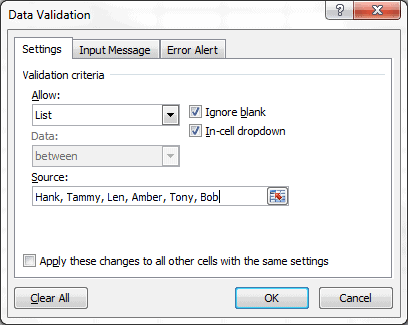
• Select the Settings tab
• In the Allow box, select List
• Click the Source box
• Type in a list of values separated by a comma
• Make sure the In-cell dropdown box is checked
• Click OK

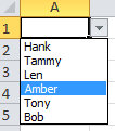
The list I created was for cell A1, which is shown below.

Excel 2010 Drop Down List

List Data Sources

Manually entering the source data for the Excel 2010 drop down list is probably the least desirable method. A better way is to put the list in a range, then refer to the range.

The same list data was put into the range J1: J6, then I changed the source reference to these cells. This is a better method than manually entering the values, but older versions of Excel require the list to be on the same worksheet. One way around this and a better solution is to give the List range a Name.

You can give the List range a Name then use it for the Source. For example, I selected the range J1: J6 then typed TheNames into the Name box, thereby creating a Named Range. On the Data Validation dialog box, I typed in =TheNames into the Source box.

Change the Reference to the Named Range

Now let’s assume that we have to add a couple more names to the list. Instead of changing every cell that references this Data Validation list, we just change the reference to the Named Range. (Choose Formulas > Name Manager, select the Named Range, change the reference in the Refers to box, then click the green arrow to make the change and click Close.)

But if the list will grow over time, changing the reference should be done automatically with a dynamic Named Range formula. We’ll do this by using the OFFSET formula.

• Choose Formulas > Name Manager
• Select New
• Type a Name in the Name box (I’ll use myNamesList)
• In the Refers to box type =OFFSET(Sheet1!$J$1,0,0,COUNTA(Sheet1!$J:$J),1)
• Click OK

Now select the cell or range with Data Validation and,

• Choose Data > Data Validation
• Select the Settings tab
• In the Source box type in =myNamesList (or the Name you created)
• Click OK

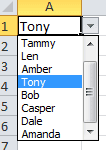
This Named Range formula is dynamic, which means the source list will expand when names are added to the list. If the list contains more than 8 values the drop-down list will have a scroll bar.

Excel – Pick from Drop Down List

Bonus Tips

One of the things we love the most about creating a drop down list in Excel is that the program reminds you to save your work before you click out. However, the program will not remind you to create a backup. If you do not have an automated backup system in place, we highly recommend implementing one. For example, you can download and save a copy locally to your desktop and USB drive. If you are using a thumb drive, store the saved copy offsite. Does this sound like overkill? Maybe. But you will not think so if you lose your first copy and then find yourself in need of it. 

How to use a drop down list in Google sheets. 

If you are not close to a device with Excel, you might have to use spreadsheets. Things in spreadsheets are simple. All you have to do in order to create a drop down list is to select the columns you need and afterward to go to Data. Then you will have to select data validation. 

In spreadsheets, data validation gives you the following criteria: List from a range, List of items, Number, Text, Date, Custom Formula, and Checkbox. Also, you can allow someone to type invalid data or to reject it by default. 

You can also create a Yes/No Drop down list, by using the criteria “List of items” and by typing in the box yes and no separated by a comma. The last step is to choose the option “On invalid data reject input”.

Another thing you can do with Google sheets is to search for the items in your list by just using a few letters from the word. This comes in handy when you have a long list of names or terms and you want to find a specified one or a group of them. 

How to Create a Drop Down List in Excel: Final Thoughts.

Now that you know how to create and use a drop down list in Excel and Google Sheets, you can have fun and do some easy exercises. Try to organize what each member of your family wants to eat for a week or use a spreadsheet as a grocery list.

With Google Sheets, you can also do some real time checkups with your friends or family members. Just share the spreadsheet with them and let them come up with the needed items for the events you are attending together. 

That’s it. We hope you enjoyed reading our article on how to create a drop down list in Excel with data validation. It’s not as hard as you might have thought.  Hopefully, you can now create a drop-down list that will meet your needs. Use as many drop lists as you need, now that you know how to make them it will only take you from a few seconds to some minutes. Anyways, Happy organizing!