To calculate a moving average in Excel, average a fixed number of observations, then move that range down one row for each new result. For three values in B2:B4, use =IF(COUNT(B2:B4)=3,AVERAGE(B2:B4),""). Copying it down gives you a rolling average while withholding results for windows with missing numbers.
The window is the important part. Three periods means three observations. Seven days means seven calendar dates. Those are only interchangeable when your data has one observation for each consecutive day. We'll use daily sales so you can see exactly which dates each result covers.
Set up one row per day
Download the moving-average example workbook to follow the formulas and chart. Its Daily Sales sheet contains the daily series, and Blank and Zero lets you compare missing values with recorded zeros.
On a sheet named Daily Sales, put these headings in A1:D1: Date, Daily sales, 3-period average, and 7-day average.
Enter 1 Oct 2026 as an Excel date in A2. In A3, enter:
=A2+1Fill A3 down through A15. This gives you one row for every date through 14 October. Enter the sales values below in B2:B15; the Row column identifies worksheet rows and isn't an extra data column.
| Row | A: Date | B: Daily sales |
|---|---|---|
| 2 | 1 Oct 2026 | 100 |
| 3 | 2 Oct 2026 | 120 |
| 4 | 3 Oct 2026 | 110 |
| 5 | 4 Oct 2026 | 130 |
| 6 | 5 Oct 2026 | 140 |
| 7 | 6 Oct 2026 | 120 |
| 8 | 7 Oct 2026 | 150 |
| 9 | 8 Oct 2026 | 160 |
| 10 | 9 Oct 2026 | 140 |
| 11 | 10 Oct 2026 | 170 |
| 12 | 11 Oct 2026 | 180 |
| 13 | 12 Oct 2026 | 160 |
| 14 | 13 Oct 2026 | 190 |
| 15 | 14 Oct 2026 | 200 |
Keep the dates in ascending order. For your own data, a blank sales cell will mean missing information; a numeric zero will mean sales were recorded as zero. Don't replace missing records with zeros just to make the calculation run.
Calculate a 3-period moving average
Leave C2:C3 empty because those rows don't yet have three observations. Enter this formula in C4:
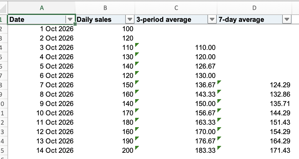
=IF(COUNT(B2:B4)=3,AVERAGE(B2:B4),"")The result is 110: (100 + 120 + 110) / 3. It sits beside 3 October, the final date in that window. This is a trailing moving average: it uses the current row and the two preceding rows.
Fill C4 down through C15. In C5, the formula becomes:
=IF(COUNT(B3:B5)=3,AVERAGE(B3:B5),"")Now the result is 120: (120 + 110 + 130) / 3. The 100 from 1 October has dropped out, and the 130 from 4 October has entered the window. That's the movement in a moving average.
The three functions each have a job:
- COUNT checks how many cells in the window contain numbers.
- IF allows the calculation only when that count is 3.
- AVERAGE calculates the mean of those three numbers.
If a window has fewer than three numeric values, the formula returns "", an empty text result that looks blank. It means incomplete window, not an average of zero. The test also withholds an average when an input is text, including a number stored as text; it doesn't explain why that input is missing or invalid.
Format C4:C15 to show two decimal places if you want a tidy display. C6 will show 126.67, while Excel retains the underlying precision. The general AVERAGE tutorial covers the ordinary mean without a moving window.
Calculate a 7-day moving average
Leave D2:D7 empty. The first complete week ends on 7 October, in row 8. Enter this formula in D8:
=IF(COUNT(B2:B8)=7,AVERAGE(B2:B8),"")Fill it down through D15. D8 averages the seven sales values from 1–7 October: their total is 870, so the average is approximately 124.29. D9 uses 2–8 October and returns approximately 132.86.
These are seven-day results because column A contains every consecutive calendar date exactly once. The formula itself only reads seven cells in column B; it doesn't inspect their dates.
If your source contains transactions only on some days, seven rows could cover ten days, two weeks, or even several transactions on one day. First arrange a daily series with one row per calendar date and put each day's sales against that date. Leave a missing daily value blank until you know what it represents. With this formula, any seven-day window containing that missing value stays blank.
The same reasoning applies to a three-month moving average: you need one observation for each consecutive month. The three-row calculation doesn't determine the reporting period for you.
Check what blanks and zeros do
An unguarded AVERAGE ignores blank cells in a range but includes numeric zeros. Microsoft documents this distinction in its AVERAGE function reference. It can change the meaning of your moving average without producing an error.
Try a separate sheet named Blank and Zero. Put Observation, Missing value, and Complete window in A1:C1, then enter:
| Row | A: Observation | B: Missing value | C: Complete window |
|---|---|---|---|
| 2 | First | 10 | 10 |
| 3 | Second | Leave empty | 20 |
| 4 | Third | 0 | 0 |
Leave B3 genuinely empty; don't type the words “Leave empty.” Put Ordinary average in A6 and Full 3-value window in A7, then add these formulas:
| Cell | Formula | Expected result |
|---|---|---|
| B6 | =AVERAGE(B2:B4) | 5 |
| C6 | =AVERAGE(C2:C4) | 10 |
| B7 | =IF(COUNT(B2:B4)=3,AVERAGE(B2:B4),"") | Appears blank |
| C7 | =IF(COUNT(C2:C4)=3,AVERAGE(C2:C4),"") | 10 |
B6 returns 5 because only 10 and 0 are numeric: (10 + 0) / 2. The zero counts; the blank doesn't. B7 stays blank because the window has only two numbers.
Column C shows what happens when the missing observation is supplied as 20. Both formulas return 10: (10 + 20 + 0) / 3. You now have three recorded values, including one genuine zero.
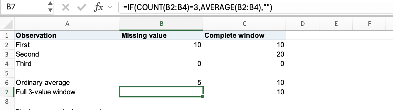
The guard makes the reporting rule explicit: require a full window before publishing an average. It doesn't fill missing information or decide whether an unrecorded day should count as zero.
Plot sales and the calculated averages
Back on Daily Sales, select A1:D15 and insert a line chart. Use column A for the date labels and columns B, C, and D as the three series. Our guide to making a line graph in Excel walks through chart setup.
Check the legend against the column headings. The sales line should start on 1 October, the 3-period average on 3 October, and the 7-day average on 7 October. Keep the leading cells in C2:C3 and D2:D7 empty rather than typing zeros; those early averages don't exist yet. If your chart draws a line down to zero, check its source cells and empty-cell settings before interpreting it.
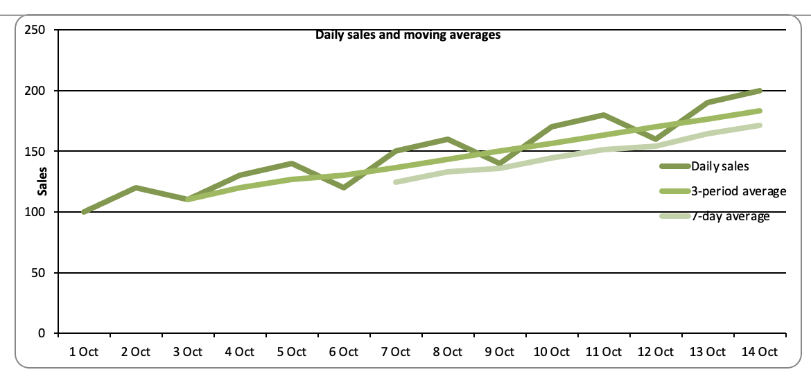
The 7-day line changes more gradually because each result combines more observations. It can also lag behind a rise in sales: D15 includes the previous six days as well as 14 October. A smoother line helps you inspect the pattern, but it doesn't predict the next day's sales.
How is this different from a moving-average trendline?
Excel also has a Moving Average trendline option for charts. That feature adds a calculated line to the chart; the method above puts the results in worksheet cells that you can inspect and reuse.
Microsoft's moving-average trendline instructions cover the platform-specific controls. A trendline period refers to data points, so setting it to 7 doesn't by itself establish a seven-calendar-day window. Don't assume its handling of missing values matches the full-window rule in these worksheet formulas.
These examples give every observation in the window equal importance. If some values need to count more than others, use a weighted average instead. Before using either result, check the latest formula's range: C15 should read B13:B15, and D15 should read B9:B15.