Your source table has five columns, but your report needs just three: Revenue, SKU, and Region, in that order. Use XMATCH to find those header names, then pass their positions to CHOOSECOLS. The report keeps every source row and follows the names when you rearrange the source columns.
With an Excel Table named Orders and your requested headers in G4:I4, enter this in G5:
=CHOOSECOLS(Orders,XMATCH(G4:I4,Orders[#Headers],0))This method needs Excel for Microsoft 365 or Excel 2024 on Windows or Mac. Microsoft lists those versions for CHOOSECOLS. XMATCH is also available in Excel 2021, but that alone isn't enough to run the combined formula.
Set up the source and report headers
You can download the example workbook to follow along with the formulas already entered. It starts with the original column order and three records; the Sorted sheet contains the sorted report. To build it yourself, use the data below.
On a sheet named Columns, paste this tab-separated example into A4:
SKU	Region	Units	Revenue	Rep
P03	West	2	50	Lee
P01	East	1	18	Kim
P02 North 4 72 RaySelect A4:E7, choose Insert > Table, and confirm that the table has headers. Name the table Orders using its Table Name field.
Enter the following headers in G4:I4. Their order is the order you want in the report:
Revenue SKU RegionEnter the formula from the introduction in G5. Leave G5:I8 available for the result and the extra row we'll add later. Keep the report outside the source Table: Excel's spilled array formulas need ordinary worksheet cells for their output.
With the three source records, the expected result in G5:I7 is:
| Revenue | SKU | Region |
|---|---|---|
| 50 | P03 | West |
| 18 | P01 | East |
| 72 | P02 | North |
The labels in G4:I4 are cells you entered; the formula supplies the data beneath them. Orders refers to the table's data rows, while Orders[#Headers] refers to its header row.
This returns all three records. If you want to enter a SKU and retrieve only its matching record, use the XLOOKUP guide for returning multiple columns instead.
Follow a header through the formula
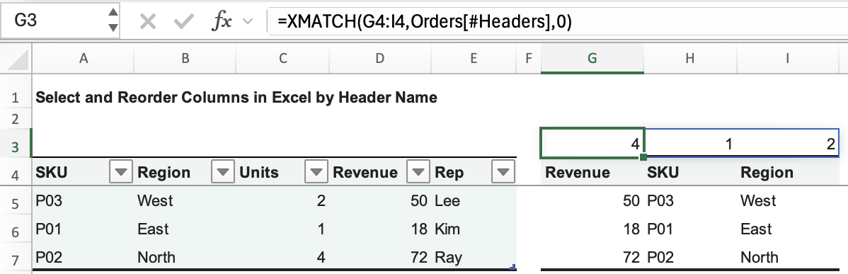
The nested formula is easier to follow when you can see the positions. Enter this in G3, leaving H3:I3 empty:
=XMATCH(G4:I4,Orders[#Headers],0)The expected values across G3:I3 are:
4 1 2Revenue is the fourth column of Orders, SKU is the first, and Region is the second. These numbers are positions within the table, not worksheet column numbers. The 0 asks for an exact match; that's also XMATCH's default. Microsoft's XMATCH documentation explains its match and search options.
CHOOSECOLS uses those three positions to return the corresponding columns in that order. You can see the same selection with fixed numbers. Copy the labels from G4:I4 to K4:M4, then enter this in K5:
=CHOOSECOLS(Orders,4,1,2)Leave K5:M8 available for this comparison. Initially, K5:M7 should match G5:I7. For the first source record, column 4 contains 50, column 1 contains P03, and column 2 contains West. Both formulas therefore produce 50, P03, West.
The difference is where the positions come from. K5 always asks for columns 4, 1, and 2. G5 asks XMATCH to find the current positions of Revenue, SKU, and Region. The trace in G3:I3 lets you see that lookup separately; G5 doesn't depend on the trace cells.
Keep the report correct when source columns move
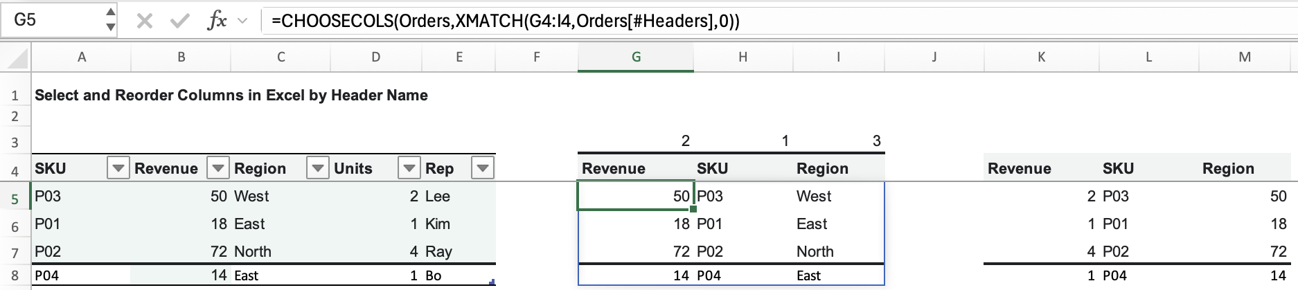
In a copy of your workbook, move Revenue so it comes immediately after SKU. For this worksheet layout in Excel for Mac, select worksheet column D and choose Cut, then select column B and choose Insert Cut Cells. This moves Revenue's header and data together, leaving this source order:
SKU Revenue Region Units RepIf you need help with the move itself, see how to move columns while keeping your data intact. In this example, the move changes the source columns' order and leaves the report cells in place. In your own workbook, check for other content in the worksheet columns before moving them.
The expected comparison is:
| Check | Before the move | After the move |
|---|---|---|
| Header positions in G3:I3 | 4, 1, 2 | 2, 1, 3 |
| First report row in G5:I5 | 50, P03, West | 50, P03, West |
| First fixed-position row in K5:M5 | 50, P03, West | 2, P03, 50 |
The fixed formula still requests the fourth column first. That column now holds Units, so its first value is 2 even though the report label above it still says Revenue. There may be no error message to warn you about the wrong field.
The header-based formula finds Revenue in position 2 and Region in position 3, keeping the requested fields under their labels.
Next, append this record to the reordered table in A8:E8:
P04 14 East 1 BoConfirm that the new row is part of Orders. The report expands to G5:I8, adding 14, P04, East in its last row. The fixed-position comparison also expands to K5:M8, but it still selects the wrong fields after the move.
Restore the original source order and three records if you want to repeat the example from the beginning.
Sort the report by SKU
Selecting columns and sorting records are separate choices. To put the report rows in SKU order, wrap the selection formula in SORT.
Create a sheet named Sorted and enter Revenue, SKU, and Region in G4:I4 again. In G5, enter:
=SORT(CHOOSECOLS(Orders,XMATCH(G4:I4,Orders[#Headers],0)),2,1)The 2 means the second column of the selected report, which is SKU. The final 1 means ascending order. Microsoft's SORT documentation describes these arguments.
With the original three records, the expected output is:
| Revenue | SKU | Region |
|---|---|---|
| 18 | P01 | East |
| 72 | P02 | North |
| 50 | P03 | West |
If you've added P04, its 14, P04, East row should follow P03. Change the formula in G5 to control the spill; individual result cells aren't independently editable.
The sort position follows the report layout. If you move SKU to a different position in G4:I4, update SORT's 2 to match its new position.
Check missing names and blocked results
If you change H4 from SKU to Product, XMATCH can't find that name in the source headers. Expect #N/A; restore SKU to correct the request. Check spelling and stray spaces before changing the formula. Keeping the error visible helps you catch a missing field instead of quietly presenting an incomplete report.
Use unique source headers. Excel Tables enforce unique column names, but a plain range can contain repeated labels. For example, put SKU, Region, Region, and Revenue in B4:E4 on a separate sheet, then enter this in an empty cell:
=XMATCH("Region",B4:E4,0)The expected result is 2: the first Region is the second cell in that range. An exact match doesn't tell Excel which of two identically named fields you intended. Give them distinct names before building the report.
For #SPILL!, check the cells the result needs. Move obstructing content out of the output area and keep the formula outside an Excel Table. For #VALUE! in a fixed CHOOSECOLS formula, check its column numbers: zero and positions beyond the source width aren't valid. Neither error should be replaced with a zero that could be mistaken for report data.