Your sales list has several rows for each product. GROUPBY can turn those transactions into one total per product, and PIVOTBY can split the same totals across regions. Put the transactions in an Excel Table, and both summaries can include new sales without rewriting the source references.
We'll use six sales totaling 190, then add another sale and check that both reports reach 200. The formulas return their results into neighboring cells, so each summary needs some empty worksheet space.
Check that your Excel supports both functions
Use Excel for Microsoft 365 with GROUPBY and PIVOTBY available. The examples here were checked in Excel for Microsoft 365 for Mac, version 16.114. Microsoft announced Current Channel availability in September 2024.
Microsoft's PIVOTBY support page also lists older perpetual editions, but that listing conflicts with the product team's guidance about new features. This walkthrough does not promise support in Excel 2021 or Excel 2024. If your installation doesn't recognize either function, use the PivotTable workflow to summarize the same source data.
Set up the sales Table
You can download the example workbook with the six transactions and both working summaries, or build it using the steps below. The download starts at the original total of 190.
On a worksheet named Example, paste this tab-separated sample into A4:
Product	Region	Sales
Binder	North	60
Binder	South	40
Binder	North	25
Notebook	North	30
Notebook	South	20
Notebook South 15Select A4:C10, choose Insert > Table, and confirm that the table has headers. Name the Table Sales using the Table Name box on the ribbon. Leave its Total Row off.
Check the source before building the summary: the amounts in C5:C10 should be numbers. The six transactions add up to 190. Binder accounts for 60 + 40 + 25, or 125; Notebook accounts for the remaining 65.
Keep E4:F7 and H4:K9 empty. These are the starting output areas, outside the Sales Table. Leave extra room beneath and to the right for more products and regions later.
Get one total per product with GROUPBY
Enter this formula in E4 and press Enter:
=GROUPBY(Sales[[#All],[Product]],Sales[[#All],[Sales]],LAMBDA(x,SUM(x)),3,1,1)The result fills E4:F7:
| Product | Sales |
|---|---|
| Binder | 125 |
| Notebook | 65 |
| Total | 190 |
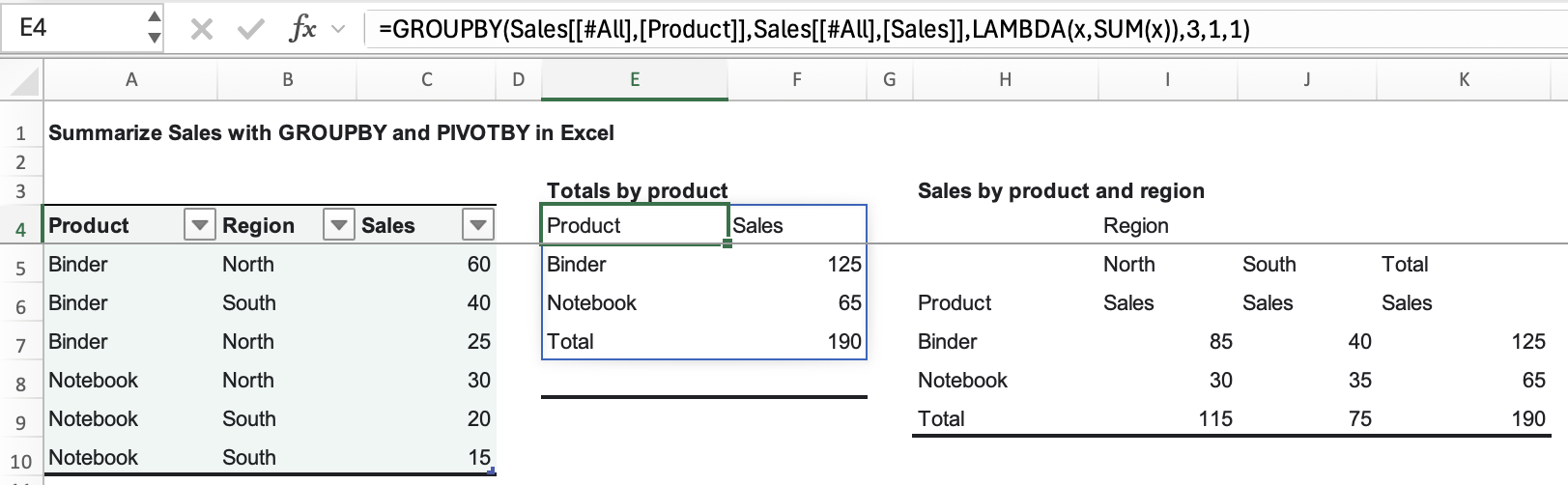
GROUPBY collects rows with the same Product and sends their sales amounts to the calculation in its third argument. In LAMBDA(x,SUM(x)), LAMBDA names the input x, and the SUM function adds the amounts in that input. You don't need to create a named function or enter a separate LAMBDA formula anywhere.
For Binder, x contains 60, 40 and 25. Their sum is 125, which appears beside Binder in F5.
The remaining settings make the report's layout explicit:
Sales[[#All],[Product]]includes the Product header and its Table column. The Sales reference does the same for the amounts. This is why the source Table's Total Row should stay off.3tells GROUPBY that the inputs contain headers and that it should display those headers.- The first
1requests a grand total. - The final
1sorts by the first grouping field, so Binder appears before Notebook.
Microsoft's GROUPBY documentation describes these arguments and the supported aggregation functions. It also shows the shorter aggregation argument SUM. This walkthrough uses the explicit LAMBDA(x,SUM(x)) form, which worked with normal formula entry in the tested Mac version; entering bare SUM there returned #NAME?.
Split each product across regions with PIVOTBY
Now enter this formula in H4:
=PIVOTBY(Sales[[#All],[Product]],Sales[[#All],[Region]],Sales[[#All],[Sales]],LAMBDA(x,SUM(x)),3,1,1,1,1)PIVOTBY groups Product down the rows and Region across the columns. It uses the same sales amounts and the same addition step as GROUPBY.
The full result fills H4:K9. It has several header rows: Region appears in I4, North, South and Total appear in I5:K5, and H6:K6 contains Product, Sales, Sales, Sales. That's expected with these header settings. The numeric part is:
| Product | North | South | Total |
|---|---|---|---|
| Binder | 85 | 40 | 125 |
| Notebook | 30 | 35 | 65 |
| Total | 115 | 75 | 190 |
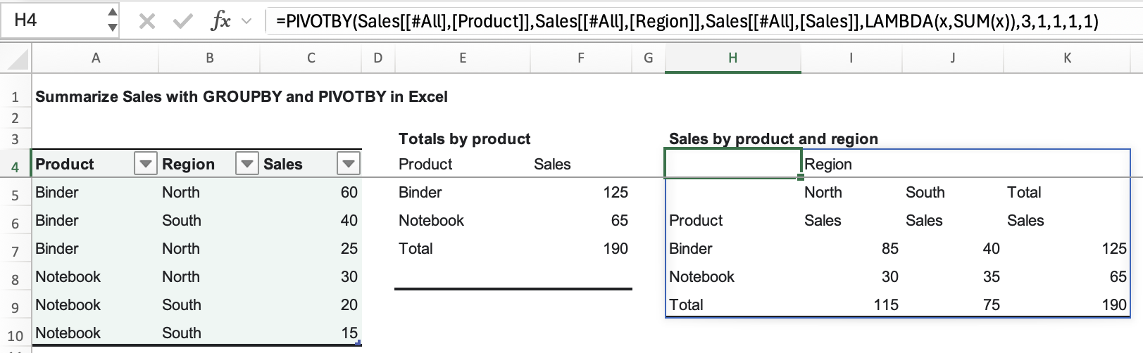
Check I7, where Binder meets North. The source has two matching transactions, 60 and 25, so this cell should contain 85. The bottom-right total in K9 should match GROUPBY's F7: 190.
After the aggregation argument, 3 tells PIVOTBY that the inputs contain headers and that it should display those headers. The next four settings specify a grand-total row, ascending product order, a grand-total column, and ascending region order. That puts North before South. See Microsoft's PIVOTBY documentation for the complete argument list.
Add a sale and check both summaries
Add this transaction in A11:C11, immediately below the source Table:
Notebook North 10Make sure Excel expands the Sales Table to include row 11. If the new row is outside the Table, resize the Table to include it; the formulas read the Table, not every nearby worksheet cell.
With automatic calculation enabled, both summaries update. Check these cells:
| Cell | What it shows | Before | After |
|---|---|---|---|
| F6 | Notebook total from GROUPBY | 65 | 75 |
| F7 | GROUPBY grand total | 190 | 200 |
| I8 | Notebook sales in North | 30 | 40 |
| I9 | North total | 115 | 125 |
| K8 | Notebook total from PIVOTBY | 65 | 75 |
| K9 | PIVOTBY grand total | 190 | 200 |
You haven't added a new product or region, so the output areas stay the same size. A new product would need another output row; a new region would also need another PIVOTBY column.
When the report looks wrong
The total is lower than expected
A complete-looking summary doesn't prove every source amount was counted. SUM ignores text and empty cells in its inputs. A sale entered as text, such as an amount prefixed with an apostrophe, can therefore be missing from the total. An empty Sales cell contributes no amount either.
In the example after adding the 10 sale, replacing C5's numeric 60 with text entered as '60 reduced both grand totals from 200 to 140. Clearing C5's contents had the same result. Both checks used the LAMBDA formulas shown above in the tested Mac version, and neither produced a formula error. To try this yourself, use a copy of the workbook and restore C5 to numeric 60 afterward.
Check the underlying amounts, especially after importing data. Changing the display format to Number alone doesn't convert stored text. Follow the steps to convert text amounts to numbers, and fill missing amounts only when you know the correct value. Then compare the product and regional totals again.
Excel shows #SPILL!
The formula needs its entire output area. Move anything blocking the cells below or beside E4 or H4, and keep both formulas outside the source Table. Edit the formula in its starting cell; the other cells belong to the returned result.
A new sale doesn't appear
First check that the new transaction is inside the Sales Table. Then check Excel's calculation setting and recalculate if the workbook uses manual calculation. A formula summary follows formula recalculation.
PIVOTBY produces a worksheet result, not an interactive PivotTable with a field list. Use a PivotTable when you want to rearrange report fields through that interface. If you're maintaining an existing PivotTable and its figures are stale, follow the separate steps for refreshing a PivotTable.