To split an existing column in desktop Excel, select the source cells and choose Data → Text to Columns. Check the preview, choose a format for each output column, and send the results to an empty destination. Those last two choices determine whether an ID keeps its leading zeros and whether date text becomes a usable date.
The original reason I used this feature was a downloaded CSV file. After opening the CSV, I had date information that Excel treated as text, but needed real dates for a graph. Text to Columns can handle the split and conversion together. The example below includes the full year so the result doesn't depend on the current system date.
Download the Text to Columns practice workbook for the source records, empty practice destinations, and expected results. The screenshots below show Excel for Mac.
Prepare the source and leave room for the result
On a worksheet named Delimited, enter these three strings in A2:A4, one per cell:
00731|2026-04-18|East
00042|2026-05-09|West
01806|2025-12-31|NorthEach string has an ID, a date in year-month-day order, and a region. The vertical bar | separates the fields.
Keep A2:A4 as the originals. Leave D2:F4 empty for the three output columns, and put ID, Date, and Region in D1:F1. Check the entire destination, not just D2: the wizard can replace existing values wherever the output lands.
Choose the splitting method based on the source:
| Method | Use it when | Example |
|---|---|---|
| Delimited | A character marks each boundary | 00731|2026-04-18|East |
| Fixed Width | Fields begin at the same character positions on every row | 00731 2026-04-18 East |
Spaces alone don't establish that data has fixed widths. Names with different lengths, for example, may need a delimiter instead. The split-names tutorial covers that separate problem and the limits of deciding which words belong together.
Split the fields at the vertical bar
- Select A2:A4, then choose Data → Text to Columns in desktop Excel.
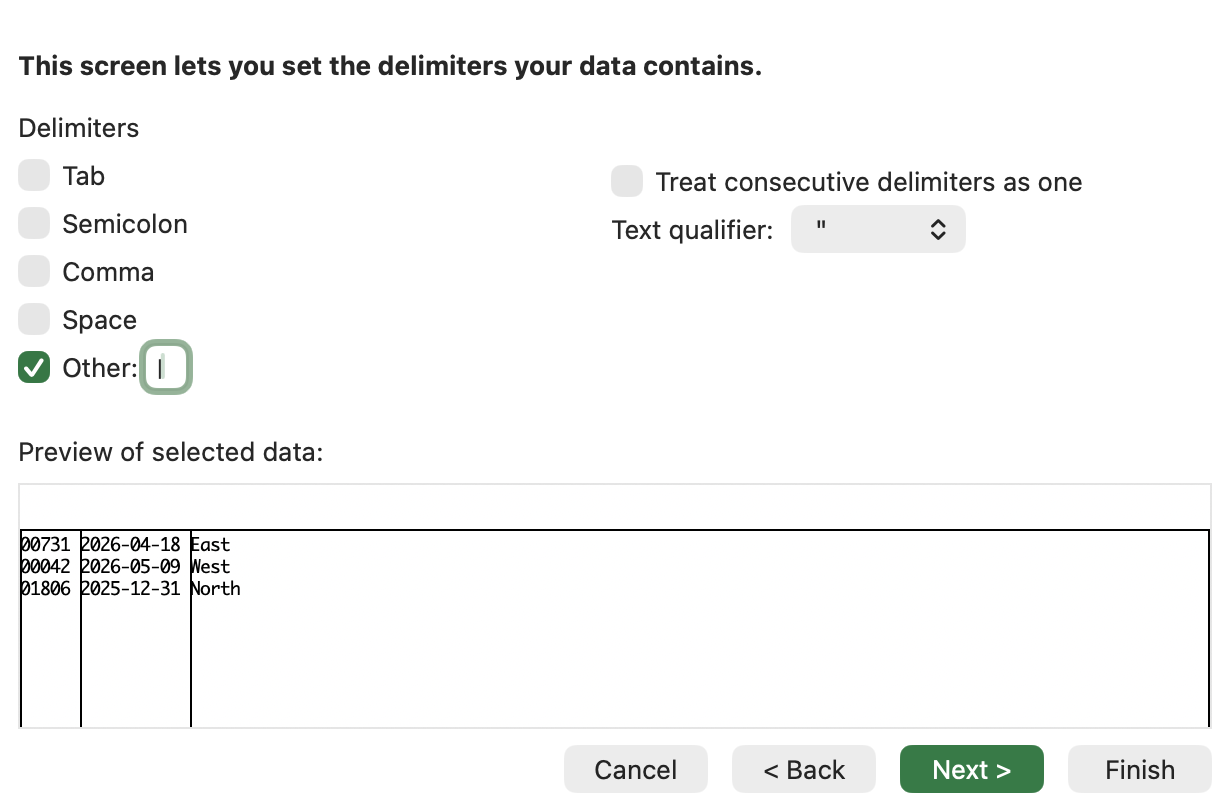
- Choose Delimited, then Next.
- Clear the other delimiter choices. Select Other and enter
|. - Check that the preview shows exactly three columns: ID, date, and region. Select Next.
This is the preview-and-destination workflow in Microsoft's Convert Text to Columns Wizard guide. The next step is where you control how Excel interprets each field.
Choose Text for IDs and Date for dates
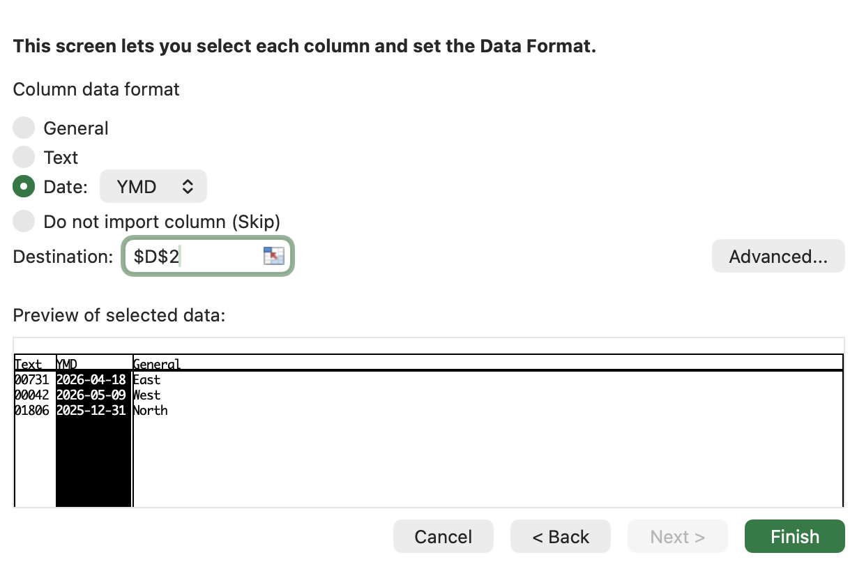
In the last wizard step, select each preview column separately before choosing its format. A setting applies to the selected column; it doesn't automatically assign the right format to all three.
- Select the first preview column, containing
00731, and choose Text. The zeros belong to the ID. - Select the second preview column and choose Date, with YMD as the source order. The input
2026-04-18is year, month, day. - Leave the third column, containing the region, as General.
- Set Destination to
$D$2. Recheck that D2:F4 is empty, then choose Finish.
If Excel asks to replace existing data, confirm that the destination is the intended range and is empty or contains only values you no longer need. Accept only after that check; otherwise cancel and choose an empty destination.
Choosing Text preserves leading zeros that are still present in the source. It can't recover digits that disappeared before the data reached A2. If an imported ID has already become 731, go back to a source that still contains 00731.
The Date option describes the order of the source date. It isn't a request for a particular display format. Choose YMD for these strings even if you normally display dates as month/day/year or day/month/year.
Check the ID and the underlying date
The first result row should contain:
| D2: ID | E2: Date value | F2: Region |
|---|---|---|
Text 00731 | April 18, 2026 | East |
E2 may display as 4/18/2026, 18/04/2026, or another date layout. Apply a date format that lets you inspect the full year. The other rows should contain IDs 00042 and 01806, with May 9, 2026 and December 31, 2025 respectively.
To check what Excel stores, work on a copy of the worksheet and temporarily change E2's number format to General. A real Excel date displays as a numeric serial; a text value such as 2026-04-18 stays as text. Restore the date format after checking. Changing the format itself doesn't convert a text date.
Then, in H2, enter:
=E2+1Format H2 as a date. It should show April 19, 2026. To check the order of the completed records, sort a copy of the output by its Date column: December 31, 2025 comes first, followed by April 18 and May 9, 2026. Include the ID and Region columns in that sort so the records stay together.

If the conversion went wrong, undo it promptly and check the source order and selected preview column. Use Cmd+Z on Mac or Ctrl+Z on Windows. A neat-looking result isn't enough if the month and day have been swapped.
For date text already in its own column, see converting a text date to a date serial number. If the date is embedded in a longer description, extracting a date with a formula may fit the source better.
Use Fixed Width when the field positions line up
On a separate worksheet named Fixed Width, put these values in A2:A3:
00731 2026-04-18 East
00042 2026-05-09 WestEvery ID uses five characters, every date uses ten, and the fields start in the same positions. Select A2:A3, start Text to Columns, and choose Fixed Width.
In the break preview, separate the five-character ID, the single space, the ten-character date, the next space, and the region. Set breaks after character positions 5, 6, 16, and 17. Excel may suggest some lines already; click at each missing position in the preview to add one. On Mac, double-click an unwanted line to delete it, or drag a line to move it. Keeping the two separator spaces as their own fields makes it clear which columns to skip.
In the final step, set the ID column to Text, both one-space columns to Do not import column (Skip), the date to Date/YMD, and the region to General. Use $D$2 as the destination on this sheet as well. Check the preview across both rows before finishing; the resulting D:F fields should match the first two delimited records.
If a date or ID has a different width on another row, those break positions won't fit it. Correct the source structure or choose a method that follows its actual separators.
Use TEXTSPLIT when the result should update
The wizard creates separate values. Changing the original string afterward won't update those results. In Microsoft 365 or Excel 2024 for Windows or Mac, TEXTSPLIT provides a formula alternative.
On the Delimited sheet, leave J2:L2 empty and enter this in J2:
=TEXTSPLIT(A2,"|")The formula spills three text fields across J2:L2: 00731, 2026-04-18, and East. Keep all three cells free; an occupied spill area prevents the result from expanding.
The date field is still text at this stage. TEXTSPLIT separates the fields without the wizard's per-column Date/YMD choice, so convert that date deliberately before using it for date calculations. Microsoft's desktop and web split guide also directs Excel for the web users to TEXTSPLIT because the web version doesn't have the Text to Columns wizard.
If another split field contains amounts with unfamiliar decimal or thousands separators, follow the text-to-number conversion guide before using them in a total. Keep the original strings until you've checked the output throughout the list. The Data Cleanup guides cover the next steps when a successful split reveals other imported-value problems.