To add a Total Row in Excel, select a cell inside your table, turn on Total Row from the table's Ribbon tab, then choose a calculation in each column you want to summarize. Choosing Sum creates a SUBTOTAL formula, so the result changes when you filter the table.
That gives us a useful starting point for a report: total the setup hours, total the number of setups, and divide one by the other. The catch is keeping that calculation correct when you filter the records—or switch the Total Row off.
Turn on the Total Row
Start with an Excel table, rather than a range that only looks like one. If you haven't converted your data yet, the table design walkthrough explains the difference.
- Select any cell inside the table.
- In Excel for Mac, open the Table tab and select Total Row.
- Click a cell in the new row at the bottom of the table, open its dropdown, and choose Sum.
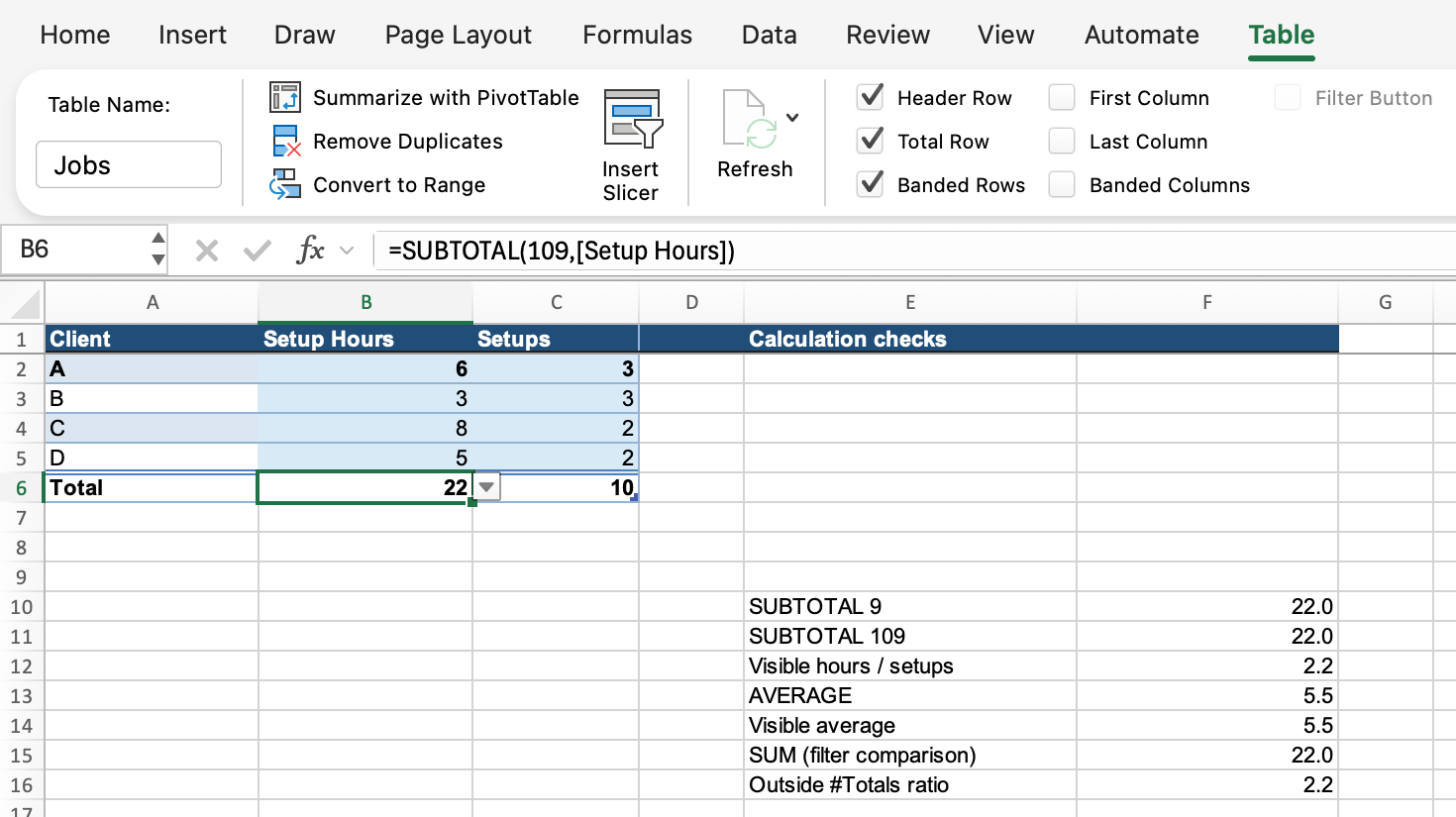
Excel for Mac: turn on Total Row from the Table tab, then choose a calculation for each column.
</figcaption> </figure>For Windows, Microsoft documents Table Design > Total Row. Ribbon labels depend on the platform; the Microsoft Total Row instructions provide the platform alternatives.
Each column has its own dropdown. You can total one column and average another, or leave a column without a calculation. For the example below, choose Sum in both numeric columns.
Choose Sum for the hours and setups
Suppose you have these four client records in a table named Jobs. Put the headings in A1:C1 and the four records in A2:C5. Setup Hours contains decimal hours, and Setups contains the number of setups completed.
You can follow along in the Total Row practice workbook, which includes the Jobs table and the calculation checks below.
| Client | Setup Hours | Setups |
|---|---|---|
| A | 6 | 3 |
| B | 3 | 3 |
| C | 8 | 2 |
| D | 5 | 2 |
With all four records visible, the Total Row shows 22 in B6 under Setup Hours and 10 in C6 under Setups. Selecting Sum in Setup Hours creates this formula:
=SUBTOTAL(109,[Setup Hours])The Setups total uses the same calculation with a different column:
=SUBTOTAL(109,[Setups])The 109 tells SUBTOTAL to add the included values. The name in square brackets identifies the table column. Inside the Total Row, Excel already knows which table you're using; outside it, include the table name, as in Jobs[Setup Hours]. The earlier formulas and structured references walkthrough explains these column references in more detail.
Notice that choosing Sum from the dropdown doesn't insert an ordinary SUM formula. That difference matters as soon as you filter your report.
Why SUBTOTAL follows a filter
Enter this formula in F15, outside the table:
=SUM(Jobs[Setup Hours])Then enter this one in F11:
=SUBTOTAL(109,Jobs[Setup Hours])Both return 22 with all the records visible. Now use the Client filter to show only A and B. Their hours add up to 9. SUBTOTAL returns 9, but SUM still returns 22 because its column reference includes all four records.
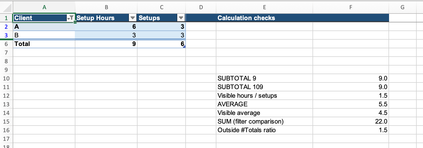
What changes between 9 and 109?
For comparison, enter one more formula in F10:
=SUBTOTAL(9,Jobs[Setup Hours])Both 9 and 109 mean “add the values.” Both leave out rows excluded by a filter. The distinction is what happens when you manually hide a worksheet row: 9 includes it, while 109 leaves it out. Microsoft's SUBTOTAL documentation describes these two groups of function numbers.
Clear the Client filter, then manually hide the worksheet row containing Client C. You have hidden 8 hours, so the formula using 109 returns 14. The formula using 9 still returns 22.
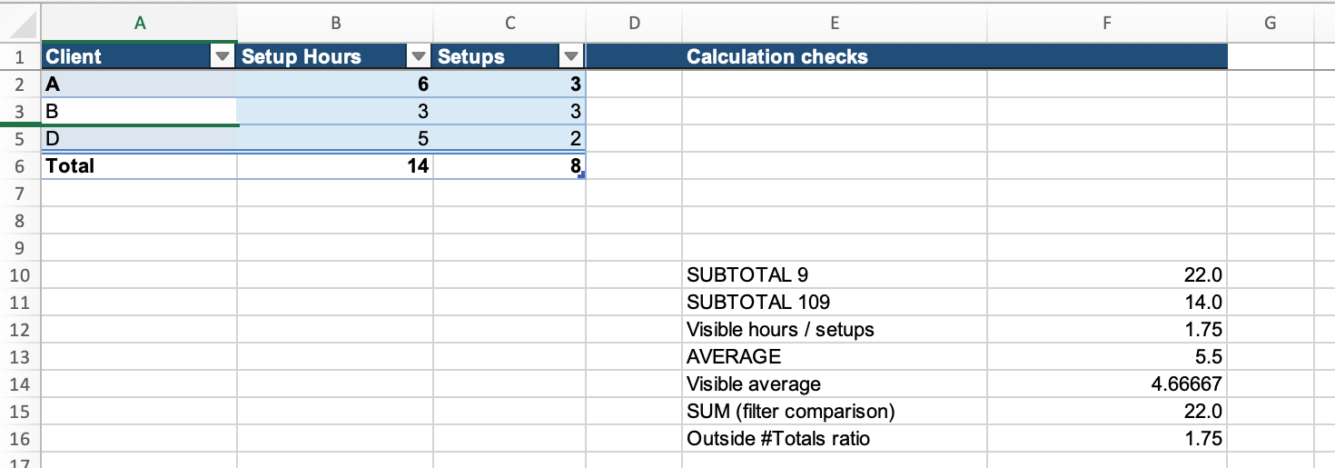
| Table state | SUM | SUBTOTAL with 9 | SUBTOTAL with 109 |
|---|---|---|---|
| All four clients visible | 22 | 22 | 22 |
| Filtered to A and B | 22 | 9 | 9 |
| Filter cleared; C manually hidden | 22 | 22 | 14 |
Unhide Client C before moving on. Filtering and hiding can look much the same on the worksheet, but they aren't the same instruction to SUBTOTAL.
Average setup hours for the visible clients
The same distinction applies to averages. These two formulas calculate the average Setup Hours value per client record. Enter the first in F13:
=AVERAGE(Jobs[Setup Hours])Enter the second in F14:
=SUBTOTAL(101,Jobs[Setup Hours])AVERAGE adds the four values and divides by four: 22 / 4 = 5.5 hours per client record. Function number 101 selects the average calculation in SUBTOTAL, excluding filtered-out and manually hidden rows.
| Table state | AVERAGE | SUBTOTAL with 101 |
|---|---|---|
| All four clients visible | 5.5 | 5.5 |
| Filtered to A and B | 5.5 | 4.5 |
| Filter cleared; C manually hidden | 5.5 | 14/3 ≈ 4.6666667 |
Choosing Average in the Total Row's Setup Hours dropdown also uses 101. Keep that dropdown set to Sum for our next calculation, though. We need total hours and total setups to calculate hours per setup.
Calculate average hours per setup
An average of the Setup Hours column answers “how many hours per client record?” Our original reporting question is different: how many hours did each setup take, on average? With 22 hours and 10 setups, the answer is 2.2 hours per setup.
Put this formula in F12, outside the table:
=SUBTOTAL(109,Jobs[Setup Hours])/SUBTOTAL(109,Jobs[Setups])The numerator adds the included hours, and the denominator adds the setups from the same records. Divide those totals to get the rate.
Filter to A and B again. The formula now divides 9 hours by 6 setups, returning 1.5 hours per setup. Clear the filter and manually hide C instead: it divides 14 by 8, returning 1.75.
A formula using ordinary SUM for both parts keeps returning 2.2 in either view:
=SUM(Jobs[Setup Hours])/SUM(Jobs[Setups])That's useful for an all-record rate, but it won't tell you the rate for the clients you've left visible. Use SUBTOTAL for both parts when you want the calculation to follow the table's filter and manually hidden rows.
If you filter out every record, the SUBTOTAL ratio tries to divide 0 by 0 and returns #DIV/0!. The same division error occurs whenever the included setups total is zero. There are no setups to divide by in that view; clear or broaden the filter and check the Setups values.
Reference the Total Row—or calculate independently of it
You can also read the two totals directly. Enter this formula in F16:
=Jobs[[#Totals],[Setup Hours]]/Jobs[[#Totals],[Setups]]With all four clients visible and both Total Row dropdowns set to Sum, it returns 2.2. Here, #Totals means the Total Row itself, rather than the table's data rows.
There is a catch: this formula depends on that row being turned on. Microsoft documents that #Totals returns null when there is no Total Row, so switching it off removes the totals this formula needs to read.
In this Excel for Mac example, the formula in F16 displayed #REF! when Total Row was turned off; turning it back on restored the result.
The earlier ratio using two SUBTOTAL calculations reads the data columns directly. It keeps working with the Total Row switched off. Use that version when someone might hide the summary row but still needs the hours-per-setup result elsewhere in the report.
Add a record and check the totals
Clear the filter and unhide every record first. Insert a new table data row above the Total Row and enter Client E, 5 Setup Hours, and 1 Setup. Make sure the new record is inside the table; Microsoft's guide to expanding a table covers adding rows.
The totals become 27 hours and 11 setups, and the hours-per-setup ratio becomes 27 / 11 ≈ 2.454545. You don't have to extend a range in the formula: Jobs[Setup Hours] and Jobs[Setups] include the new table record.
Remove that added record if you want to return to the four-client example. With all four clients visible, check for 22 hours, 10 setups, and 2.2 hours per setup.