To turn several Excel columns into one list, enter =TOCOL(B4:D5) in an empty cell. With 11, 12, 13 in the first source row and 21, 22, 23 in the second, the result runs down one column: 11, 12, 13, 21, 22, 23. Each source value gets its own cell.
The choice to make is which direction Excel should read your grid. You can read across each row first, as above, or finish one source column before moving to the next.
Microsoft lists TOCOL and TOROW for Excel for Microsoft 365 and Excel 2024, on both Windows and Mac. See its TOCOL documentation for the supported versions and arguments.
Put the grid into one column
Download the example workbook to compare both scan directions on List and the different empty-looking entries on Blanks.
To build the example yourself, create a sheet named List and paste these tab-separated values into B4:
11	12	13
21 22 23The source fills B4:D5. Leave F4:F9 empty, select F4, and enter:
=TOCOL(B4:D5)The expected result is six cells, from F4 to F9:
11
12
13
21
22
23Excel reads B4 → C4 → D4, then B5 → C5 → D5. It puts those values into the output in that order. You enter the formula once, in F4; the neighboring results belong to that formula. This is called a spilled array.
Keep headings outside the source reference unless you want them included as list entries. TOCOL reads the cells you give it; it doesn't identify which entries are headings.
If you want to swap rows and columns while keeping a two-dimensional report, use Paste Transpose or a TRANSPOSE formula. Flattening a grid also doesn't join its values into a single text cell, or preserve source field names beside each value as an unpivoted table would.
Read down each source column first
Suppose each source column is a separate list and you want all of column B before column C. Leave H4:H9 empty and enter this in H4:
=TOCOL(B4:D5,0,TRUE)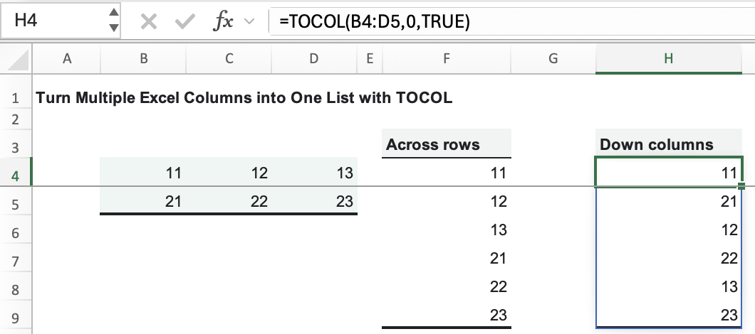
The expected result changes to:
11
21
12
22
13
23This time Excel reads B4 → B5, then C4 → C5, then D4 → D5. Compare F5 with H5: F5 is 12, while H5 is 21. That second entry is a quick way to check which scan order you're using.
The final argument, TRUE, selects this column-first scan. Leaving it out, or using FALSE, reads across rows. The middle argument, 0, keeps all source entries. It occupies the second argument position so that TRUE can go in the third.
Decide what counts as an empty entry
A cell can look empty for several different reasons. Before changing the formula, separate these cases:
| Source content | What it means for your list |
|---|---|
| An untouched cell | A truly blank source cell; the default TOCOL formula returns a zero in its position. |
The number 0 | An actual numeric value, retained when you ignore blanks. |
A formula returning "" | Empty text with zero characters, retained when you ignore blanks. This is a formula result, not an unused source cell. |
| One typed space | Text containing one character, also retained when you ignore blanks. It may look empty, but ignoring blank cells isn't a whitespace cleanup step. |
To see why that distinction matters, create a separate sheet named Blanks. Enter 11 in B4, leave C4 untouched, enter 0 in D4, and enter 21 in B5. In C5, enter:
=""In D5, type one space and press Enter. You now have four different cases in the same small range. Don't type the word “blank” into C4; that would turn it into a text entry.
In F4, start with the default formula:
=TOCOL(B4:D5)The truly blank C4 produces a zero, while D4 supplies its own numeric zero. Those two zeros have different origins. Hiding every zero would also hide the valid source value.
To omit truly blank cells, enter this in H4:
=TOCOL(B4:D5,1)Here are the results from the example in Excel for Mac. Empty text and one space below describe the invisible entries; Excel doesn't display those labels in the output.
| Position in list | Keep everything: F4:F9 | Ignore blanks: H4:H8 |
|---|---|---|
| 1 | F4: 11 | H4: 11 |
| 2 | F5: 0, from blank C4 | H5: 0, from numeric D4 |
| 3 | F6: 0, from numeric D4 | H6: 21 |
| 4 | F7: 21 | H7: empty text |
| 5 | F8: empty text | H8: one space |
| 6 | F9: one space | No sixth entry |
With 1, only the untouched C4 is skipped. The result still contains the numeric zero, the empty text from C5, and the space from D5. F8 and H7 contain text of length zero; F9 and H8 contain text of length one. Those last entries may look alike on the sheet, but they aren't the same value.
A space is easy to enter without noticing. Inspect the source before deciding that a blank-looking output is an error; changing TOCOL's blank setting won't remove that space.
Choose whether to keep errors
The second argument controls both blank and error handling:
| Second argument | Entries omitted |
|---|---|
0, or omitted | None |
1 | Blank cells |
2 | Error values |
3 | Blank cells and error values |
To compare all four settings, make a copy of the Blanks sheet and name it Error QA. Leave C4 untouched, D4 as numeric zero, C5 as empty text, and D5 as one space. Replace B5, which currently contains 21, with:
=1/0B5 now shows #DIV/0!. Leave K20:K25 empty and enter this in K20:
=TOCOL(B4:D5,0)The result has six entries, including the error. Change the second argument to 1 to skip the blank source cell while keeping the error. Then replace the K20 formula with this to omit the error while keeping the blank's position:
=TOCOL(B4:D5,2)Finally, replace it with this to omit both the blank and the error:
=TOCOL(B4:D5,3)Compare each result with these sequences, listed from top to bottom. As before, empty text and one space describe entries that look empty in the cells.
| Second argument | Number of entries | Result sequence |
|---|---|---|
0 | 6 | 11, 0, 0, #DIV/0!, empty text, one space |
1 | 5 | 11, 0, #DIV/0!, empty text, one space |
2 | 5 | 11, 0, 0, empty text, one space |
3 | 4 | 11, 0, empty text, one space |
Only 2 and 3 skip the error. Neither removes the empty text or the space. With 3, the remaining zero is the real numeric value from D4.
Check source errors before choosing either option. Omitting this division error makes the list shorter; it doesn't repair B5. Keep the default behavior when errors need to remain visible for correction. To reset your test sheet, put 21 back in B5. The downloaded workbook keeps the original, error-free example; Error QA is a separate sheet you create for this comparison.
Return one row instead
On the List sheet, leave B13:G13 empty and enter this in B13:
=TOROW(B4:D5)The expected horizontal result is:
11 12 13 21 22 23TOROW changes the output orientation. Its default still reads across the source rows. To read down the source columns while returning one horizontal row, replace the formula in B13 with:
=TOROW(B4:D5,0,TRUE)The expected sequence across B13:G13 is now 11, 21, 12, 22, 13, 23. Microsoft's TOROW documentation describes the same blank, error, and scan-order arguments used by TOCOL.
Flattening preserves repeated entries. If your next task is to keep only distinct values, see the UNIQUE function reference.