To switch rows and columns in Excel, copy your cells and use Paste → Transpose. If the result needs to follow changes in the source, use a TRANSPOSE formula instead. The important choice is whether you're making a one-time copy or a report you'll keep using.
Suppose your regions run down the left of a small sales report, but you need the regions across the top. We'll make both versions from the same cells, then change one sales figure to see the difference.
If you only want to change the order of existing columns, use the guide to moving columns in Excel. Transposing changes the direction of the whole range: rows become columns, and columns become rows.
If every value should go into a single column, see how to turn multiple columns into one list.
Start with a small report
Download the example workbook to compare the source, pasted copy, and linked formula side by side. It opens with the completed comparison: North's Q1 is 135 in the source and formula result, while the pasted copy still shows 120. To replay that change, set C5 back to 120, then change it to 135 again. The Notes sheet explains the source and the two results.
On a worksheet named Transpose, enter this data in B4:D6. Include the labels when you select the range; they need to travel with the figures.
| Cell row | B | C | D |
|---|---|---|---|
| 4 | Region | Q1 | Q2 |
| 5 | North | 120 | 150 |
| 6 | South | 90 | 0 |
The zero in D6 is a real sales figure. Leave it in place. Give B4:D4 a fill color so it's easy to recognize the original headings.
After transposing, the layout should read:
Region  North  South
Q1      120    90
Q2 150 0North's Q2 figure is still 150. Its position has changed, but the relationship between the region, quarter, and amount hasn't.
Make a one-time copy with Paste Transpose
This first example contains typed labels and numbers, so the pasted result can stand on its own.
- Select B4:D6 and choose Copy on the Home tab.
- Select F4. Check that F4:H6 is empty before pasting; existing contents there would be overwritten.
- On the Home tab, open the arrow beside Paste and choose Transpose.
- Check F4:H6 against the result above. G6 should contain North's Q2 figure, 150.
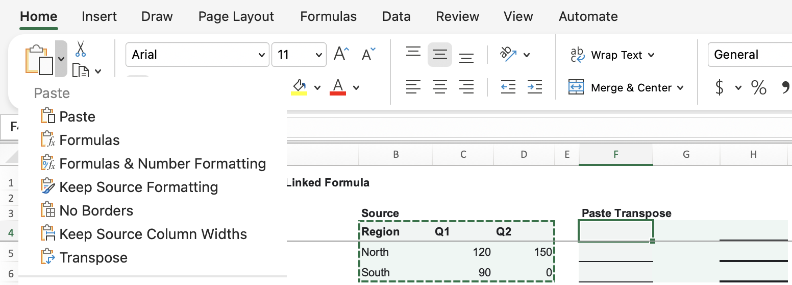
These are the steps in Microsoft's Mac transpose instructions. Start with Copy: the Transpose command doesn't work with Cut.
The header formatting moves with the pasted cells. In the example workbook, the fill and bold text from B4:D4 appear down F4:F6, where Region, Q1, and Q2 now sit.
The destination must have room for the reversed dimensions. Our three-row, three-column source still needs three rows and three columns. A two-row, three-column source would need three rows and two columns. Choose a destination away from the source so you can compare both.
If the source contains formulas
A pasted transpose of formulas needs an extra check. Standard Transpose paste can copy the formulas and adjust their cell references; it isn't a guarantee of fixed values. Select a pasted formula and check the formula bar before relying on its result.
For a fixed snapshot of formula results in Excel for Mac:
- Copy the source formula cells and select the top-left destination cell in an empty area.
- Press Control+Command+V to open Paste Special.
- Select Values, check Transpose, and choose OK.
The difference matters even with a small range. In a separate example, A15 contained 7, B15 contained =A15, and C15 contained =B15. Copying B15:C15 with All + Transpose to F15:F16 changed the formulas to =F14 and =F15. With F14 empty, both returned 0. Using Values + Transpose at I15:I16 instead produced two literal 7 values, with no formulas to adjust.
Microsoft's paste options guide distinguishes copying formulas from pasting their calculated values. If the references are the problem, our guide to absolute and relative cell references explains which parts can change when you copy a formula.
Keep the result linked with TRANSPOSE
For a report that should follow the source, leave J4:L6 empty. In Microsoft 365 Excel, select J4, enter this formula, and press Enter:
=TRANSPOSE(B4:D6)The result should fill J4:L6 with the same labels and figures as the pasted version. Excel calls this spilling: one formula returns several values into the neighboring cells.
The formula result keeps the destination's formatting. In this workbook, J4:L6 stays plain; the source's header fill and bold text aren't copied across. Format the output cells separately if you want them to match your report.
B4:D6 is the range to turn around. Its first row becomes the result's first column; its North row becomes the result's North column. Check K6: it should contain 150, corresponding to D5 in the source. Microsoft's TRANSPOSE documentation explains the range argument and the different entry methods.
Keep the source cells. This result depends on them. To change the formula, select J4, the top-left cell of the result, rather than trying to edit one of its neighboring output cells.
Change one figure to compare the two methods
Now change C5 from 120 to 135. This is North's Q1 figure. Compare these three cells after calculation:
| Location | Cell | Expected value |
|---|---|---|
| Source report | C5 | 135 |
| Pasted transpose | G5 | 120 |
| Formula transpose | K5 | 135 |
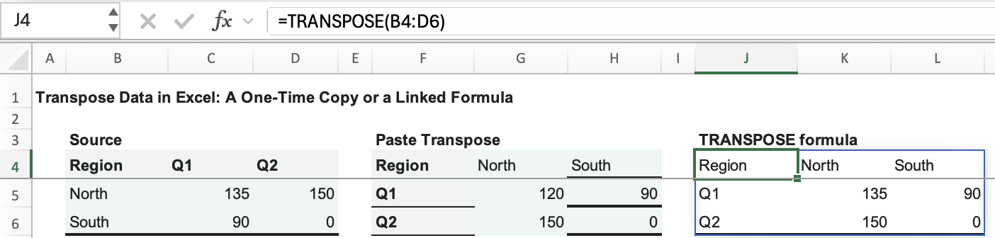
The pasted copy keeps the number you copied earlier. The formula reads the changed source. Use the paste method when you need that fixed copy; use the formula when the source remains the place where you'll enter corrections.
The range in this formula is specifically B4:D6. If you add another region below it, update the reference to include that new row and leave room for an additional output column.
Keep blank cells and genuine zeros separate
An empty source cell and a zero can look the same after transposing. In this example, clearing D5 makes its linked output, K6, display numeric 0. The genuine zero in D6 still appears as 0 in L6.
A formula that returns empty text is a different case. Enter this in D5:
=""K6 now looks blank, while L6 still displays the genuine zero. D5 contains a formula returning empty text; it isn't a truly empty source cell.
Don't hide every zero to make the report look cleaner. That would also hide South's actual Q2 figure. Check the corresponding source cell first, and restore 150 in D5 when you've finished this comparison.
Fix a blocked result or an unavailable command
J4 shows #SPILL!
Check whether something is already in J4:L6, apart from the formula in J4. A value in K5, for example, blocks the result. Move the blocking entry somewhere safe, or clear it if you no longer need it. The formula can then fill the range.
Place the formula outside an Excel Table as well. Spilled results need ordinary worksheet cells, even when their source data is in a Table. See Microsoft's explanation of spilled array behavior for these restrictions.
Transpose isn't available for an Excel Table
Microsoft's Mac instructions note that the paste command isn't available when the source is an Excel Table. Use the formula in an empty area outside the Table if you want to keep the Table. Converting it to a normal range is another option, but that changes the source structure as well.
Use the right entry method in older Excel
Older Excel versions without dynamic arrays require you to select the entire destination before entering TRANSPOSE. For this example, select J4:L6, type =TRANSPOSE(B4:D6), and confirm it as a legacy array formula.
Microsoft documents Ctrl+Shift+Enter for legacy array entry on Windows. Excel adds the surrounding braces itself; don't type them. For a source that isn't square, reverse its dimensions when selecting the destination: two rows by three columns becomes three rows by two columns.
In Microsoft 365 Excel, use the single-cell entry described above instead: select J4, enter the formula, and press Enter.