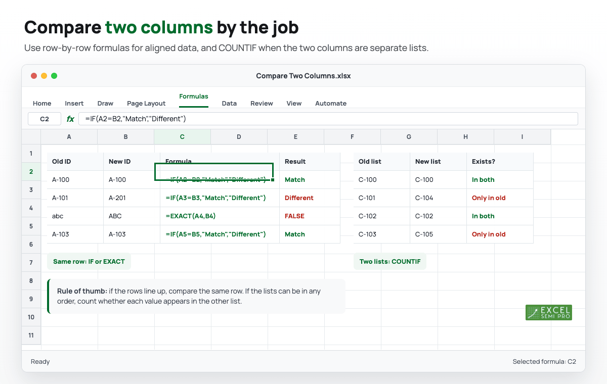
To compare two columns in Excel, use =A2=B2 when the values should match row by row. If you want readable labels, use =IF(A2=B2,"Match","Different"). If the two columns are separate lists and the order may be different, use COUNTIF instead.
The right method depends on the job. Comparing two cells in the same row is different from checking whether every value in one list appears somewhere in another list.
| Task | Best method | Example formula |
|---|---|---|
| Compare values in the same row | Direct comparison | =A2=B2 |
| Show labels instead of TRUE/FALSE | IF | =IF(A2=B2,"Match","Different") |
| Compare text with case sensitivity | EXACT | =EXACT(A2,B2) |
| Check if a value from column A exists anywhere in column B | COUNTIF | =COUNTIF($B$2:$B$20,A2)>0 |
| Return related data from the matching row | XLOOKUP | =XLOOKUP(A2,$E$2:$E$20,$F$2:$F$20,"Missing") |
| Return a spill list of missing values | FILTER plus COUNTIF | =FILTER(A2:A20,COUNTIF(B2:B20,A2:A20)=0,"None") |
You can download the compare two columns example workbook to practice the row-by-row formulas, unordered list checks, and lookup examples from this guide.
Microsoft also has a support article on comparing data in two columns to find duplicates, but the examples below split the problem by the way people actually use the worksheet.
Compare Two Columns Row by Row
Use this when row 2 in column A should match row 2 in column B, row 3 should match row 3, and so on.
Enter this formula in C2:
=A2=B2
Then copy it down.
Excel returns:
TRUEwhen the two cells match,FALSEwhen they are different.
Example:
| Old ID | New ID | Formula | Result |
|---|---|---|---|
| A-100 | A-100 | =A2=B2 | TRUE |
| A-101 | A-201 | =A3=B3 | FALSE |
| A-102 | A-102 | =A4=B4 | TRUE |
This is the fastest method for simple side-by-side checks.
Mark Matches and Differences with IF
TRUE and FALSE are useful, but labels are easier to scan in a worksheet.
Use this formula in C2:
=IF(A2=B2,"Match","Different")
Then copy it down.
The IF function checks the comparison first. When A2=B2 is TRUE, it returns Match. When the comparison is FALSE, it returns Different.
Use labels when you plan to filter, sort, or share the result with someone who does not need to read formula logic.
Compare Two Columns with Case Sensitivity
The normal formula =A2=B2 is not case-sensitive. In many worksheets, that is fine.
For example, Excel treats these as equal:
="abc"="ABC"
If letter case matters, use EXACT:
=EXACT(A2,B2)
EXACT returns TRUE only when the text matches character by character, including uppercase and lowercase letters. It is useful for product codes, imported IDs, short labels, and other text where abc and ABC should not be treated as the same value.
To show labels instead of TRUE/FALSE, wrap it in IF:
=IF(EXACT(A2,B2),"Exact match","Different")
Highlight Matches or Differences with Conditional Formatting
If you want the worksheet itself to show differences, use Conditional Formatting.
To highlight row-by-row differences:
- Select the range you want to check, such as
A2:B20. - Go to Home > Conditional Formatting > New Rule.
- Choose Use a formula to determine which cells to format.
- Use this formula:
=$A2<>$B2
- Choose a fill color.
- Click OK.
The $A2<>$B2 formula means: compare the value in column A with the value in column B on the same row. The column letters are locked, but the row number adjusts as the rule moves down the selected range.
To highlight matches instead, use:
=$A2=$B2
If your real goal is to remove duplicate records after you find them, use this article only for the comparison step and then review How to Delete Duplicates in Excel.
Compare Two Unordered Lists with COUNTIF
Use this method when column A and column B are separate lists and the order does not matter.
For example, column A may contain last month's customer IDs, while column B contains this month's customer IDs. You want to know whether each old ID still appears in the new list.
Enter this formula in C2:
=COUNTIF($B$2:$B$20,A2)>0
Then copy it down.
The COUNTIF function counts how many times the value from A2 appears in B2:B20.
- If the count is greater than zero, the value exists in both lists.
- If the count is zero, the value from column A is missing from column B.
For labels, use:
=IF(COUNTIF($B$2:$B$20,A2)>0,"In both","Only in A")
Use absolute references like $B$2:$B$20 so the lookup range does not move when you copy the formula down.
Find Values in Column A That Are Missing from Column B
If you have Microsoft 365, Excel 2024, or Excel 2021, you can return the missing values as a spill list with FILTER:
=FILTER(A2:A20,COUNTIF(B2:B20,A2:A20)=0,"No missing values")
This returns every value from A2:A20 that does not appear in B2:B20.
Use this when you want a clean exception list instead of a helper column. If Excel returns a #SPILL! error, clear the cells below the formula so the results have room to spill.
Return Matching Values with XLOOKUP
Sometimes comparing two columns is only the first step. You may also want to return related information from the matching row.
Suppose:
A2:A20contains IDs you want to check,E2:E20contains the master ID list,F2:F20contains the status you want to return.
Use XLOOKUP:
=XLOOKUP(A2,$E$2:$E$20,$F$2:$F$20,"Missing")
This searches for A2 in the master list and returns the matching status. If the ID is not found, it returns Missing.
For a fuller lookup walkthrough, see the XLOOKUP function in Excel guide.
Common Mistakes When Comparing Two Columns
Extra spaces make values look different
Two cells can look identical but still fail a comparison because one has a leading or trailing space.
If imported text is suspicious, test with:
=TRIM(A2)=TRIM(B2)
TRIM removes extra spaces from the start and end of text. If lookup formulas are failing because of hidden text problems, the troubleshooting guide on VLOOKUP not working with text values covers related cleanup patterns.
Numbers stored as text may not compare the way you expect
An ID such as 00125 may be text on purpose. A quantity such as 125 should usually be a number. Before forcing a conversion, decide whether the leading zeros matter.
Blanks can create false matches
If both cells are blank, =A2=B2 returns TRUE. If blanks should not count as matches, combine the comparison with AND:
=IF(AND(A2<>"",B2<>"",A2=B2),"Match","Check")
COUNTIF is not case-sensitive
COUNTIF treats abc and ABC as the same value. If case matters across lists, use a helper column with EXACT for the specific rows you need to test.
FAQ
What is the easiest way to compare two columns in Excel?
Use =A2=B2 when the two columns should match row by row. Use COUNTIF when you need to check whether values from one list appear anywhere in another list.
How do I compare two columns and show Match or Different?
Use:
=IF(A2=B2,"Match","Different")
Copy the formula down for the rest of the rows.
How do I compare two columns for duplicates?
Use:
=COUNTIF($B$2:$B$20,A2)>0
This checks whether the value in A2 appears anywhere in column B.
How do I compare two columns and highlight differences?
Use Conditional Formatting with the formula =$A2<>$B2 for row-by-row differences. Select the range first, then create a formula-based rule.
Which formula should I use for case-sensitive comparison?
Use:
=EXACT(A2,B2)
Wrap it in IF if you want labels instead of TRUE/FALSE.