columns Tips & How To's • Excel Semi Pro

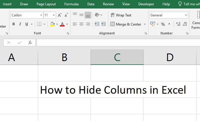
How to Hide Columns in Excel

April 30, 2023June 19, 2019

Did you know that there are several ways you can learn how to hide columns in Excel? While most people know about this Microsoft software feature, there are a couple of things that you might not be aware of. For example, you can hide or unhide more than one column at a time. If the …

Image that shows how to freeze cells in Excel.

How to Freeze Cells in Excel So Rows and Columns Stay Visible

April 30, 2023June 14, 2018

Have you ever worked in an unorganized spreadsheet? We have to admit, there is nothing more frustrating. When you scrolled down the endless rows, chances are, you couldn’t see your headers anymore. How are you supposed to keep track of where you are plotting data? This is where knowing how to freeze cells in Excel …