Understanding the Datetime Handling in Excel
In Excel, date-time values are a blend of date and time, stored as serial numbers. Excel represents dates as sequential serial numbers where each number corresponds to a specific date, starting from January 1, 1900. Time is represented as fractional parts of a day. For instance, 0.5 represents noon, as it is halfway through the day. This unique representation allows Excel to perform calculations and manipulations on date-time values. However, extracting specific components, like time from a date-time value, requires a certain level of understanding of these serial numbers and the functions Excel offers to manipulate them.
I have a worksheet that tracks start and stop times for different events throughout the day, all during the week. Sometimes I have to pull out the Time of Day, irrespective of the Date, with the TIME function.
The TIME function has three arguments: Hour, Minute, Second. I could use =TIME(11,30,0) in a cell to get 11:30 AM, but I want to convert a Date-Time number so let's look at an example.
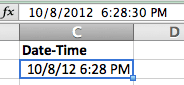
In cell C2 I have the Date-Time value 10/8/12 6:28:30 PM.
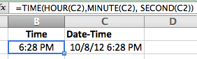
In cell B2 I enter the formula =TIME(HOUR(C2),MINUTE(C2), SECOND(C2)) to pull out the time value. Notice that the HOUR, MINUTE, and SECOND functions are used to extract values for the Hour, Minute, and Second arguments. The TIME Function puts these into a nicely formatted time value of 6:28 PM.
Now the Time values can be used independently of the Date.
Note: You don't see the 30 seconds in cell B2 because of the default cell formatting for Time in my spreadsheet.
A Shortcut Formula [UPDATE]
I had a reader comment about an easier formula so I will include it in this post. Thanks JMarc.
A Date-Time serial number, with General formatting, shows up as an Integer.Fraction. You don't normally see this on your spreadsheet as Excel will automatically format Date-Time numbers as, well, Date-Time numbers.
The screen shot below shows the Date-Time number and its serial number equivalent with General formatting. Both underlying numbers are identical, the cell formatting is the only difference.
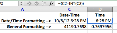
The INT function returns the integer portion of a number. If we use the Date-Time number and subtract the integer portion, that leaves us with the fractional portion, which is the Time. The formula =C2-INT(C2) will return the number 0.769795602.
Reformatting the cell to a Time format will allow the fraction to show as a Time value.
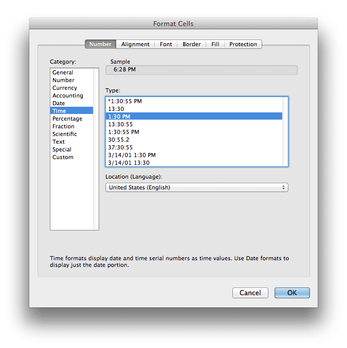
Changing the cell formatting gives us the time value 6:28 PM.