I recently found myself with a new, loaner laptop and a brand new copy of Excel 2003 as my default spreadsheet program. This was fine until I realized there were a number of things “missing.” Like shortcuts and settings that I’ve changed over the years to make Excel serve me, instead of the other way around.
So here’s my list of things I do to “normalize” Excel 2003.
Full Menu’s
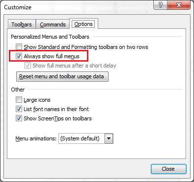
My number one pet peeve with Excel is they “automatically customize menus and toolbars based on how often you use the commands.” But my question is, “How do new users know what menu commands are available if they’re hidden?”
I like to use “full menus” so you see ALL menu commands each time each time you click a menu. This is a standardized approach; you see the same thing each time you click a menu.
Here’s how it’s done:
-
Right click the toolbar
Click Customize…
Click the Options tab on the Customize dialog box
Check Always show full menus
Click Close

General Options
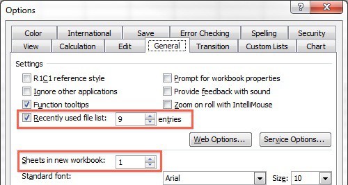
I have only two recommendations here: maximizing the recently used file list and minimizing the number of worksheets in a new file.

Recently used file list (9)
I like to set the recently used file list to the maximum number. In Excel 2003 that number is nine. This saves you time when searching for a recently used file.
Here’s how it’s done:
- Choose Tools > Options then click the General tab on the Options dialog box. Change the Recently used file list to 9 and make sure there’s a check in the check-box.
Sheets in new workbook (1)
When creating a new spreadsheet file, how many sheets do you actually use? How many times have you looked over a spreadsheet file from someone else and clicked on those bank sheets to see if they contained anything?
Remember the days when a new file had 16 worksheets as the default? Excel 2003 has just three. That’s two to many. I like to set the number of worksheets in a new file to one. If I need another, they’re easily created.
Here’s how it’s done:
- Choose Tools > Options then click the General tab on the Options dialog box. Change the Sheets in new workbookto 1.
Shortcuts on the Toolbar
These custom toolbar buttons are necessary when using Excel 2003: Paste Values, Freeze Panes, Current Region, Auto Filter, and Pivot Table. You can easily customize the toolbar to add these and more.
![]()
For each addition to the toolbar you’ll need to access the Customize dialog box. The long way is to choose View > Toolbars > Customize… or the short way is to right-click a toolbar and select Customize… from the pop-up menu.
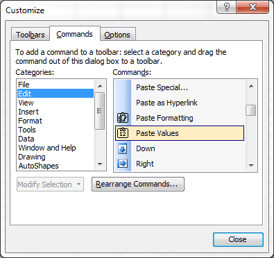
Once the Customize dialog box is open, select the Commands tab. Now your ready. Here’s my favorite custom toolbar commands.
Paste Values
The very first custom toolbar command icon I put up. Indispensable. Well, almost.
Here’s how it’s done:
- In the Categories pane select Edit. In the Commands pane scroll down and find Paste Values. Click and hold the left-mouse button down while dragging the icon to a toolbar.

Freeze Panes
Another indispensable toolbar command button shortcut icon for anyone who works with lots of data in proper tables.
Here’s how it’s done:
- In the Categories pane select Window and Help. Scroll down until you find Freeze Panes. Click with left mouse button, hold and drag to the toolbar.
Select Current Region
Here’s a neat button that allows you to find the shape of a data region by selecting it for you automatically. Better than the keyboard shortcut Ctrl+Shift+asterisk (*). Reminds me of the CurrentRegion property in VBA.
Here’s how it’s done:
- In the Categories pane select Edit. In the Commands pane scroll down to the bottom and find Select Current Region. Click and hold with the right-mouse button while dragging to a toolbar of your choice.
AutoFilter
A great button to save you some time when filtering tables. If the active cell is on the header row it simply turns on the filter. However, if you select a cell in the data that contains something you want to filter, clicking the AutoFilter will turn on AND filter that selection for you. A one step process that saves time.
Here’s how it’s done:
- Select Data from the Categories pane. Click the AutoFilter command with the left mouse button, hold and drag to a toolbar.
PivotTable
This command serves to initiate a PivotTable from a data table. It also brings up the PivotTable and PiotChart Wizard when you are working on an active PivotTable.
Here’s how it’s done:
Select Data from the Categories pane. Scroll down to the bottom of the Commands pane and find PivotTable and PivotChart Report icon. Left-click, hold and drag to a toolbar.
More Stuff
Find your favorite command not shown on a Toolbar and load it up. Pronto!
