Tag Archives: Excel 2008

A Dynamic Dependent Drop Down List with a Horizontal Table Reference

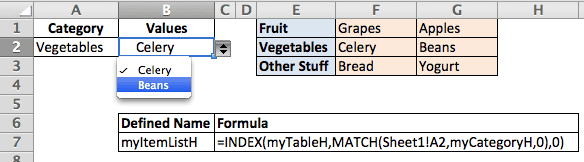
I received a comment asking if a dynamic dependent drop-down list in Excel could have a list where the “table headers were actually rows and not columns?” Since I’ve already detailed how this is done in the article mentioned above, I’ll keep this short. The screen shot below is what I’ll be referencing. At the end of the post I’ll give a link to the file I used.

Conditional Drop Down List (Excel)

There are two named ranges,

myCategoryH

myTableH

that refers to range F1:G3.

A defined name, myItemListH, is created with the following formula =INDEX(myTableH,MATCH(Sheet1!A2,myCategoryH,0),0) that will return a row that is matched by the contents of cell A2.

In cell A2, add a Data Validation list with the source being =myCategoryH. In cell B2, add a Data Validation list with the source being =myItemListH in the conditional drop down list from Excel.

Now you’re done.

Cell A2 will give you a drop-down list of Fruit, Vegetables, or Other Stuff. And cell B2 will read the value in cell A2, match and return the proper row number, and return an array of values for that row.

Two Ways to Use the INDEX Function to Return an Array

This is a simple case of using the INDEX function in a slightly different way. Normally, to return column 2 of a named range, you would use the following formula =INDEX(myTable,0,2). The zero means: return all rows (of column 2).

If you want to return row 2 of the named range you would use =INDEX(myTable,2,0). Here the zero means: return all columns (of row 2).

This comes from the Help section of the INDEX function where in Excel 2011 it reads:

If you set row_num or column_num to 0 (zero), INDEX returns the array of values for the entire column or row, respectively. To use values returned as an array, enter the INDEX function as an array formula in a horizontal range of cells for a row, and in a vertical range of cells for a column. To enter an array formula, press ⌘+RETURN.

Practical Considerations

Adding to each category list across columns is problematic. For one thing adding more data to the table will require inserting a column within the table range to avoid renaming the range. Obviously a standard Excel “Table” won’t work with this type of list. And if you have a very large spreadsheet the number of columns will become limiting long before the number of rows would.

Download the File

Horizontal-Dynamic-Dependent-Drop-Down-List.xlsx

How to Update a List or Range without OFFSET

I avoid the use of Volatile Functions, especially OFFSET, which is commonly used to update a list or range. They can slow down the operation of your workbook. For very large workbooks with lots of data, it can be significant and irksome.

Worksheet cells that use Data Validation for a drop-down list can simplify the input process, or be used to limit the available choices. But the list needs be expandable. Here are two primary ways to keep your data validation list automatically updated, without having to resort to using the OFFSET function.

Update Your List Range with VBA

Put your data validation drop-down cell on one worksheet and the reference list range on another worksheet. Example: Sheet1 contains a cell with data validation. Sheet2 contains a data range (the list) that is given a defined name of myList. Add some VBA code in the Sheet2 Deactivate routine to update the named range.

Private Sub Worksheet_Deactivate() Dim rng As Range Set rng = Sheet2.Range("myList").CurrentRegion Set rng = rng.Offset(1, 0).Resize(rng.Rows.Count - 1, rng.Columns.Count) rng.Name = "myList" End Sub

This is an event-based programming technique, which I commonly use with Excel 2003.

Use Some Table INDEX Magic

This is a variation of the same thing, but no VBA programming is warranted. Instead, use a Table for your reference list data. Then create a defined name with the INDEX Function, and use that name for the data validation list.

Tables automatically update their ranges when expanded and the INDEX function will too. Example: Create the defined name myListFormula and use =INDEX(Table1,0,1) as the formula. Then when setting the data validation list, use =myListFormula as the list reference.

Example Worksheet

I’ve put together a workbook with the two examples listed above. The first technique, with VBA, uses two worksheets: Lookup 1 and Data 1. The Data 1 worksheet has the VBA code, which updates the named range when deactivated. You can add or subtract to this list and the data validation list on the Lookup 1 sheet will automatically be updated.

Both Lookup sheets have data validation in cell A2, which is a list of names. I’ve added another column for the city that uses a formula to get the right value from the list.

Lookup 1 Sheet

Data 2 Sheet with VBA Code

The second example uses Lookup 2 and Data 2 worksheets. The Table is on the Data 2 worksheet. When you add or subtract data from this Table and the defined name myListFormula will automatically update the data validation list on the Lookup 2 worksheet. Be sure to look at the Define Name dialog box (on the Mac) or the Name Manager (Windows) to see the INDEX formula.

Download the file: Data_Validation_List_Update.xlsm

Since there is no OFFSET function, updating at random intervals, in either of these examples, I can rest easy. That’s one less thing to slow down your worksheet.

Select Excel’s Used Range on a Mac

I recently read a good blog post over at Contextures about selecting the actual used range on an Excel sheet, both manually and with VBA. However, using Excel on a Mac makes you keenly aware that there’s no Home button.

The used range on a worksheet starts with cell A1 and ends with the last used cell in the worksheet. This “last cell” is not always apparent, but easily found. Just use the keyboard shortcut CONTROL + G to bring up the Go To dialog box.

Click Special… which will bring up the Go To Special dialog box.

Select Last cell and click OK.

The last cell may sometimes surprise, because Excel considers cell formatting as being “used” so you may see blank cells that are way outside your data range. Tip: Sometimes you can delete the seemingly extra rows and columns outside your data range and it will reduce the file size.

Select the Used Range by Navigating Back Home

Once you find the last cell, you can then hold the Shift key down and click cell A1 to select the entire range. Of course if you can’t see cell A1 in the current window there is no Home button on the Mac to help you out. (Major bummer)

The next best thing is to hold the COMMAND + Shift keys down while you tap the left arrow and up arrow keys until you reach cell A1. This can be simple, or time-consuming depending upon size and shape of your worksheet.

Selecting the Used Range

To select the entire used range with VBA is a simple matter. Choose Tools > Macro > Visual Basic Editor, then choose View > Immediate Window, and type activesheet.usedrange.select inside the immediate window and hit enter.

Create a Macro to Select the Used Range

You can also create a macro to select the entire used range by opening the VBA Editor, inserting a Module, and entering the following code.

Sub ActiveSheetUsedRange() ActiveSheet.UsedRange.Select End Sub

Or you could get fancy with this code.

Sub SelectUsedRange() Dim rng As Range Set rng = Range("A1").SpecialCells(xlCellTypeLastCell) Range(Cells(1, 1), rng).Select End Sub

Add a Keyboard Shortcut for the Macro

To make things simpler to run the macro, you can enter a shortcut. Just choose Tools > Macro to bring up a dialog box.

To add a shortcut, select a macro and click Options… which will bring up the Macro Options dialog box.

Enter a shortcut key by clicking inside the Shortcut key box and pressing a key on the keyboard. I pressed the “u” key on the keyboard, and consequently the keyboard combination is shown as Option + Cmd + u, as you can see in the screen shot. (Depending on the key, you may also include COMMAND, Control, Shift into your shortcut.)

Enter a description if you wish, and then click OK. Select the Cancel button on the Macro dialog box to make it disappear.

Now you can run the macro by simply using the keyboard shortcut Option + Cmd + u.

Note: This macro will not work if a Chart sheet is selected.

Used Range verses Actual Used Range

The actual used range might be different than the used range. Meaning that some blank cells that are formatted might be included in the used range. Most likely you will only want to deal with a range that has some actual values. This would be the actual range.

Please refer to the aforementioned blog post over at Contextures to see a couple of different examples of code that you can use to select the actual used range. These examples are short and use the VBA FIND function to get the job done.

An Excel Crossroads – Mac and Windows

I bought a MacBook Pro and installed Windows 7 with Boot Camp Assistant so I could access the “normal” Excel. This was important to me at the time because I was doing Excel development work in versions 2003, 2007 and 2010 on a Windows PC.

I love my MacBook Pro, which I consider my computer of the future. It’s great for dealing with Photos, Movies, Music, and all of my iOS devices.

I purchased the Mac versions of Excel (2008 and 2011) but they seem like a mixture of the three Excel versions mentioned above, and can be very frustrating at times. There are a few things missing in the latest Excel Mac version, like the Name Manager and the Evaluate Formula dialog box, to name just two.

Despite these shortcomings, I’m seriously thinking about selling my desktop PC and going exclusively with the Mac. That’s the crossroads I’m at right now. Letting go of the PC, but keeping the Windows versions of Excel.

My Hangups

BootCamp allows me to run Windows, and the Excel versions I need, but is very restrictive in the sense that I have to shut down my Mac, then restart with BootCamp to run Windows 7. This is a real pain in the you-know-what.

There are other problems with running Windows on a Mac. For instance, I haven’t been able to get my Apple Magic Mouse to work with Windows 7. (Go figure.) And using Dropbox was the best way to get Excel files between Windows 7 and Mac OS X.

My Saving Grace

All of those issues were solved when I purchased the Parallels Desktop software for Mac. Now I can switch to Windows without having to shut down Mac OS X Lion. That’s just plain awesome!

I’m still getting used to how Parallels works, but this software is easily worth the purchase price. And my Apple Magic Mouse, just works.

Parallels Desktop on my MacBook Pro

Here’s a screen shot of the Parallels Desktop open on my MacBook Pro. You can see that I have Microsoft 2010 (Windows) open, but I want you to notice that I also have the Finder dialog box open.

I dragged the Card Size Lookup.xlsx file from Finder onto the Excel 2010 (Windows) program and it opened. I then made a change to the spreadsheet and saved it. The file was saved back on my Mac from whence it came. This is the miracle of modern technology.

I still have lots of testing to do but it looks like the Parallels Desktop has made my life much, much easier. I know now which way to turn at the crossroads.

Microsoft Query Incompatible with Mac OS X Lion [Updated]

The other day I read an article on how to prepare my MacBook Pro for Lion, the new Mac OS X coming out this month, and discovered that any application that requires PowerPC is incompatible with Lion and will not work. See update at the end of this post.

So I followed the instructions to check all the installed programs on my MacBook Pro and was surprised to find that Microsoft Query will be incompatible. This will affect any Excel for Mac versions you might have on your computer — 2004, 2008, 2011.

I would venture a guess that 99.4% of all Excel users have never used Microsoft Query, but I’m one who does and thought this might be significant to a select few. (Notice that Open XML for Excel and Charts uses PowerPC too.)

Microsoft Query allows you to pull data into an Excel spreadsheet from “behind the wall,” so-to-speak, of a database or ERP system. I made a career out of doing this very thing. Getting data that others could not.

In Microsoft 2010 (Windows) the new PowerPivot can replace Microsoft Query but in Excel for Mac there’s no replacement.

Excel for Mac users should beware, Microsoft Query is an incompatible app in the upcoming Lion upgrade for Mac OS X.

[UPDATE]

Since I wrote this post Microsoft updated their Office 2011 software. If you have Microsoft Office version 14.1.2 or later Microsoft Query has been updated to Intel, as you can see in the screen shot below, instead of PowerPC, and will now work on your Mac with OS X Lion.

Thanks to J. Monroe who pointed out the update by Microsoft in a comment.

That Damn Delete Key in Excel for Mac

I have no earthy idea why it took me so long to figure out how to delete the contents of a cell or range in Excel for Mac. Ever since I bought my MacBook Pro I’ve known the Delete key on a Mac isn’t really a Delete key.

I mean, since my background is with Windows, I have ingrained knowledge on how the Delete Key works on a computer. Ingrained, I tell you.

But all of that knowledge was shattered upon getting a Mac.

Where Is the Excel Delete Button on Mac

After some consternation, I learned where is the delete button on a Mac. To press the delete button on Mac computers you have to hold down the fn key and the Delete key at the same time when you want to delete something on a Mac. (Skip to video)

After a while, you get used to the idea that the Delete key on a Mac is really a backspace key and using fn+Delete gives you the real Delete key action. 🙂

Of course if you’re a long time Mac user you probably think I’m cuckoo. But hey, this is my blog, think what you like. I’m not the only one who’s decided to start using a Mac after a lifetime of Windows abuse use.

Excel for Mac

Anyway, when using Excel on a Mac — I’ve got versions 2008 and 2011 — you run into a learning curve with all the unusual shortcut keys, function keys (1, 2), and menu and ribbon things that are different from the Windows version of Excel. So there’s a tendency to forget about how the Delete key works on a Mac.

I mean, this is Excel we’re talking about here. Hitting the Delete key is supposed to delete the contents of the active cell, for cryin’ out loud.

In Excel for Mac it does that, but the cursor also gets stuck inside the cell in edit mode. You have to hit the enter key to finish deleting the contents, but this act also moves the active cell to the next cell down.

And if you’ve selected a range and hit the Delete key, the active cell contents are deleted and the cursor is stuck inside the cell in edit mode. You have to hit the Enter key, which does nothing but take you to the next cell. The range contents are still there, with the exception of the active cell.

Not the kind of behavior that occurs in Excel for Windows.

How to Delete Cell and Range Contents in Excel for Mac

The trick is to remember that fn+Delete is really a keyboard shortcut to the Delete key on a Mac. Then the world rights itself and the planets align. Frustration abates. You’ve finally found the magic. Your mojo is back!

Watch this 54 second video to see what I’ve been babbling about for the past 454 words.

YouTube link

Create a List in Excel 2008

I was surprised to find a List Wizard in Excel 2008 (Mac) because Excel 2007 (Windows) has Tables, and had already been out for nearly a year when Excel 2008 was released.

Here I’ll walk you through the process of setting up a List in Excel 2008 but won’t go into every detail because, as you’ll soon see, there are lots of features in the List Wizard. I’ll start with the same data table from my last post.

To create a List in Excel 2008, select your existing data table and choose Insert > List…, and the List Wizard will appear.

Step 1 of 3 wants to know Where is the data is for your list? and has correctly selected the range and guessed that My list has headers. It also wants to know Where do you want to put the list?

I leave all of these selections unchanged and select Next > to move along to Step 2 of 3.

Here you can select each column in the List and change the Column name and Data Type.

The Settings button takes you down-the-rabbit-hole, so to speak, and brings up a Column Settings dialog box.

Here you can also change the Column Name and set the Data Type but you can also choose the cell Formatting, set up Conditional Formatting, and Data Validation.

Click Formatting… to bring up the Format Cells dialog box. Select the Condition Formatting… button to bring up the Conditional Formatting dialog box. Click the Validation… button to bring up the Data Validation dialog box. Having these three features available is rather amazing. (I’ll forgo the screen shots of each dialog box.)

There are three more options on the Column Settings dialog box. Formula, Default value and Unique values only. If you select Calculated Column for the Data Type, then the Formula box becomes active and you can enter a formula for that column. If you select the check box for Default Value that box becomes active and you can enter a value that will appear each time a new row is generated. Selecting the check box for Unique Values will then only allow unique values to be entered into that particular column. You get a warning when trying to enter a duplicate value.

Remember, all of these features can be performed on every column of data in the List.

Clicking Next > brings you to Step 3 of 3 in the List Wizard.

Here you can change the List name. If you select the box for Autoformat list after editing the AutoFormat… button becomes active and will bring up a dialog box if selected.

Finally, you can also click the box to Show totals row, and Show List visuals to On or Off or leave the default setting of Auto.

Click Finish to create the List.

Notice the floating toolbar with List controls. The bottom three on the right toggle AutoFilters, Total Row, and Visuals. The latter being the exaggerated border around the List that shows when the list is active.

Along the top row of this toolbar you can access the List Wizard, Column Settings, insert a column, or row, and access AutoFormat.

Then there’s the List drop-down menu (second row, first item) that gives you lots of options.

The menu item Remove List Manager is used to convert the List to a range.

Finally, there is an arrow head on the right side, in the middle of the toolbar that you can click with your mouse to bring up what looks to be a navigation menu.

When adding a List to Excel 2008 you can utilize numerous features that seem to be quite extensive.

Give Your List a Defined Name – Oh Wait, Don’t Bother

For all the List features you get in Excel 2008, the most disappointing thing is that when you give the List a Defined Name, Excel will not automatically expand the associated range when you add data to the List.

I selected the List range, chose Insert > Name > Define… and gave my List the name TableOne, then clicked OK.

I entered another row of data and the Defined Name TableOne still refers to the same range, cells A4:C7.

This is surprising to me because in Excel 2003 (Windows) you can give your List a Defined Name and Excel will automatically expand the range as you add more data.

The Repeat Command in Excel for Mac

Adding the Repeat command icon to the Quick Access Toolbar in Excel for Windows is a simple process that I explained in a blog post last week. Excel for Mac — 2011 or 2008 — doesn’t have a Quick Access Toolbar, but you can customize the toolbars and menus.

Add the Repeat Icon to the Standard Toolbar

Right-click the toolbar and select Customize Toolbars and Menus…

At the top of the dialog box select Toolbars and Menus
Select the Show checkbox for the Worksheet Menu Bar
In the Worksheet Menu Bar click Edit

Select Repeat and while holding down the Control key, drag to the Standard Toolbar

Click OK

Strangely enough, if you select Commands at the top of the Customize Toolbars and Menus dialog box, then select Edit from the Categories window, there is no Repeat command in the commands window. This is why I thought it didn’t exist in Excel for Mac.

The Three Different States of the Repeat Icon

The Repeat icon becomes active and has color when the current command can be repeated. It will be grayed-out if the current command can’t be repeated. After there’s been an Undo action, the Repeat icon will change to a Redo icon.

Turn on Toolbar ScreenTips

There’s an option to show shortcut keys in the toolbar screen tips that’s nice to have turned on. It shows the keyboard shortcut for the Repeat command to be Cmd+6.

Right click the Standard Toolbar
Select Customize Toolbars and Menus…
Click the Show shortcut keys in ScreenTip checkbox

Click OK

What Version of Excel am I Using?

If you’re curious about the version of Excel you’re using and don’t know how to go about it, you’ve come to the right place. It could be as simple as selecting the Help Menu and clicking About Microsoft Office Excel, but then again, maybe not. The five options below will help you sort things out.

Excel for Windows

If you’re using a Windows computer, chances are you’re using one of the three most recent versions of Excel.

Excel 2003

Select the Help menu, then click About Microsoft Office Excel.

This also works with earlier versions of Excel (2002 and 2000).

Excel 2007

Select the Office button and click the Excel Options button, then select Resources from the left-hand pane and click the About button.