Fat Fingers on the Space Bar – A Conditional Formatting Example

I had the distinct pleasure of helping a colleague this week, because he fat-fingered the space bar whilst entering data in a spreadsheet then couldn’t figure out why there were #VALUE! errors on the Pivot Report. I used some conditional formatting to solve the problem and save the day.

But to be fair, data entry errors are pernicious and can happen to anyone. And a lot of VBA programming is written to alert users of problems with input data. The example I’ll use here isn’t quite the same as the original but will illustrate the problem of having a space character entered into a cell, then having it used in a formula to generate an error.

The Problem with the Space Character

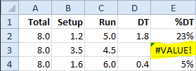
In the spreadsheet below, hours are entered by manufacturing in different buckets to determine where time was spent during the shift. Total hours equal the sum of Setup, Run and Downtime (DT) hours. The percentage of downtime is calculated in the %DT column by taking the downtime hours (DT) and dividing by the Total hours. Zeros are not a required entry.

My fat-fingered friend happen to bump the space bar on several of his entries and I’ve re-created that in cell D3, which looks to be empty but contains a space character. This bothersome fiend is like the invisible man, you suspect something is near but you can’t see anything. Yet the evidence, in this example at least, is right in front of us by virtue of the #VALUE! error in cell E3.

By a process of elimination we can tell from the %DT formula (=D3/A3) that cell A3 appears to be okay with the value 8.0 so that leaves cell D3, which appears to be empty. However it requires closer inspection to find the space character.

If we Edit the cell (F2 in Windows Cmd+O in Mac) we can usually tell by the cursor position that there is a space, but when cell alignment is centered this becomes problematic. We could simply hit the delete key to clear the contents of the cell, but we need to detect the presence of the space character in some manner so we can fashion a solution for alerting the user to the fat-finger snafu.

Finding the Solution

Using the  formula =LEN(D3) returns 1 and confirms something unseen is there. Using the formula =CODE(D3) returns 32, which is the numeric code for the space character. And using the formula =ISTEXT(D3) returns TRUE, which is, in essence, why the #VALUE! error is returned by the formula.

My solution is to encode the data range in the DT column with Conditional Formatting so that when the space bar is inadvertently pressed, leaving behind an invisible space character, the cell background becomes a rose color to get the attention of the user. Of course I need to inform the user of this fact, so I’ll put a comment in the column header for posterity.

Detect the Space Character with Conditional Formatting

To select the data range I activate cell D2, type D2:D10000 into the name box and press enter.

Choose Home > Conditional Formatting > New Rule then select the Rule Type: Use a formula to determine which cells to format. Next type the formula =ISTEXT(D2) into the Format values where this formula is true box.

Click the Format button to bring up the Format Cells dialog box, click the Fill tab, then select a background color of your choice and click OK. The New Formatting Rule dialog box should look something like this:

When you are satisfied click the OK button for the changes to take effect.

Please notice that the formula uses the topmost cell in the range with a relative reference. This allows all cells in the range to have this conditional formatting feature.

This solves our data entry problem with fat-fingers on the space bar.

Revisit Your Conditional Formatting

Once Conditional Formatting is in place we tend to forget all about it until there needs to be some changes to the conditional part or the range needs to be expanded. The first question that arises is “what was the range I formatted with conditional formatting?”

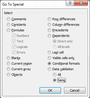
To locate the original range, select any cell that you know has the conditional formatting and use the keyboard shortcut Ctrl+G then click the Special button on the Go To dialog box. Now click the radio button for Conditional formats on the Go To Special dialog box then select the radio button for Same and click OK.

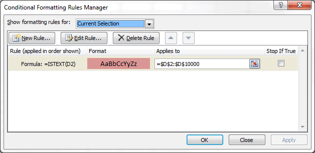
Now that the entire conditional formatting range is selected, choose Home > Conditional Formatting > Manage Rules to bring up the Conditional Formatting Rules Manager where you can change the range or edit the formatting rule or add a new rule.

You can also delete the original formatting rule should you have skinny-fingers and never unintentionally tap the space bar.