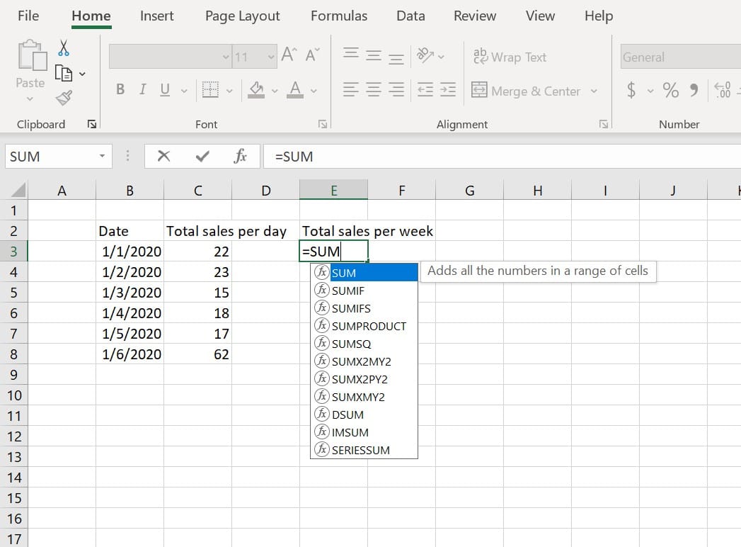
Silver laptop with excel display

The History of Microsoft Excel: How It Came to Be

Most of us are familiar with the Microsoft application Excel. It has become so popular and synonymous with data and spreadsheets that we often forget that elegant programs such as Excel did not always exist. And they did not always exist in their current format. Let's take a look at the history of Microsoft Excel to see how this beautiful data crunching software became what it is today.

Great things usually start out as something small, and in the technology world, they are usually created to solve a problem. We will learn that that is extremely true for the spreadsheet programs that we see out on the market today and especially true for the history of Microsoft Excel. We will look at how a student at Harvard Business School was looking to solve his problem of performing analysis for a case study, and that led to the creation of one of the most popular, flexible, and widely used spreadsheet programs in the world today.

What Is Microsoft Excel?

Excel Tables

Image via pixabay.com

Microsoft Excel is a spreadsheet application that was first launched by Microsoft Corporation in 1985. In order to perform mathematical functions on the data, the program organizes the data into columns and rows. This can then be manipulated through formulas which allow users to input and analyze large sets of data. Furthermore, it offers numerous automation capabilities so that users can compute large sets of data repeatedly. As we'll learn, this feature, when first introduced, gave Excel an advantage over other spreadsheet software available.

In addition, the software offers a variety of features that help users better visualize and share data. Users can easily create 3-D charts, drawings, outlines, and more to share their data analysis with others. Excel also integrates with other Microsoft Office suite programs, giving users the ability to easily share information through different programs and in different formats. This is especially useful for using data in reports and presentations created in Microsoft Office and PowerPoint.

Popular Features of Microsoft Excel

Employee learning on microsoft image

Image via pixabay.com

The uses of Microsoft Excel are practically limitless -- especially when you combine it with the accompanying Office Suite Programs. We could create a never-ending list, but let's take a look at the top 10 features of Microsoft Excel. These are features that will help you improve your ability to analyze data for your personal use or for your business.

  • Efficiently model and analyze almost any data
  • Zero in on the right data points quickly
  • Create data charts in a single cell
  • Access your spreadsheets from virtually anywhere
  • Connect, share, and accomplish more when working together
  • Take advantage of more interactive and dynamic PivotCharts
  • Add more sophistication to your data presentations
  • Do things easier and faster
  • Harness more power for building bigger, more complex spreadsheets
  • Publish and share through Excel Services

These are just the start of what you are able to do with this well-designed piece of software. It is a great tool for data analysis and can be used for both personal and business use. Its flexibility is one of its key features that have lead to its popularity throughout the history of Microsoft Excel.

History of Microsoft Excel Up Until This Point

Excel spreadsheet icon

Image via pixabay.com

It is hard to talk about the history of Microsoft Excel without talking about the entire history of spreadsheet applications and software. Let's start where it all began: Harvard Business School. In 1978, Harvard Business School student Dan Bricklin needed to perform an analysis for his case study. At the time, he had two options: complete the analysis by hand or use a clumsy mainframe program. Bricklin envisioned creating something akin to the blackboard in the classroom where data could be compiled, displayed, and computed.

By the fall of 1978, he had created the first working prototype of his vision and called it VisiCalc. It was capable of manipulating matrices of 5 columns and 20 rows. It could perform basic arithmetic operations, instant automatic recalculation, and scrolling. It was a far cry from modern-day spreadsheet programs and software, but it was the program that started it all.

After the introduction of VisiCalc in 1978, other spreadsheet programs began to appear on the market. Each had their own merits and values but a few stand out as becoming more popular than others. In 1982, Microsoft released its first spreadsheet software, Multiplan. During the same year, Lotus Development Corporation released its spreadsheet software Lotus 1-2-3. Lotus 1-2-3 was capable of iteratively solving circular references, integral charting, graphing, and rudimentary database operations. These features made it a popular choice for MS-DOS users at the time.

Noticing their loss in the spreadsheet market, Microsoft introduced the first version of Excel in 1985. At first, it was only available on Apple, Inc.'s Macintosh computer. Being the first to use a graphical interface and pull-down menus it made it easy for users to use the software with the point and click capabilities of a computer mouse. The software also offered strong graphics and fast processing.

Later, in 1987, Microsoft released a version of Excel that could be used on their new Windows Operating System. By 1988, Microsoft Excel was beginning to outsell its main competitor Lotus 1-2-3. Lotus Development Corporation was slow to release a Windows version of Lotus 1-2-3 and Excel quickly became the popular spreadsheet software of the Mid-1990s. In 1993, Microsoft released Version 5.0 of Excel which contained the Visual Basic Applications (VBA), more commonly referred to as macros. This created unlimited possibilities for automation that helped propel Excel's popularity.

Excel continued to grow in popularity with later versions of the software. Later versions offered more features and capabilities making it easier to use. Upgrades included toolbars, outlining, drawing, 3-D charts, numerous shortcuts, and automation features. These features made it the ideal program for data computation and analysis because it could easily adapt to any business process.

Improvements to the Original

person typing on silver MacBook

Image via unsplash.com

In 1995, Microsoft released Version 7.0 of Excel, more commonly known as Excel 95. It was the first 32-bit version of Excel and while no external changes were made, it offered more stability and faster performance. In 1997, Microsoft introduced versions of Excel that featured the paperclip office assistant, validations, and a new interface for VBA developers. Later, with Excell 2000, Microsoft introduced an improved clipboard, capable of holding multiple items at one time, and introduced the Excel Self-Repair.

In 2003, Microsoft released Excel 2002 as part of the Office XP suite. In addition to allowing more shareability between the Microsoft programs, this new version of Excel allowed users to recover data in the event of a computer crash. In 2007, Microsoft redesigned the user interface of Excel and its sharing features. It made it easier to move smoothly between other Microsoft Office Suite programs such as Word and PowerPoint.

Later, in 2010 and 2013, Microsoft made major upgrades to the Excel program. New features included extended image capabilities, improved pivot tables, the ability to customize the ribbon, more conditional formatting options, PowerView, FlashFill, and new functions. These features continue to make Excel an easy-to-use platform for data analysis.

Conclusion

person holding clear and blue ballpen

Image via pexels.com

Today, Excel is familiar, flexible, and widely used around the world for both personal and business use. As we look to the future, it is clear that cloud-based computing is on the rise. More and more people are using it to increase their accessibility to their data and collaborations. There is no doubt that given the history of Microsoft Excel, this popular program will continue to look for new ways to innovate and make data analysis simple and easy for everyone to use.

Microsoft continues to make upgrades and additions to Excel that make it more powerful than ever. These additions include PowerPivot, which is used to access larger data sets. They have also increased the row and column limit from 64,000 to 1 million. Microsoft also has plans to develop the integration of Excel with CTP Hadoop connector for SQL server. This development will provide for better integration with older technology as well as providing seamless integration for newer technology. This creates the huge benefit of a more expansive dataset usage capability — something of great value as data becomes the leading currency of the modern world.

As more and more businesses are moving toward cloud-based computing for the accessibility of their data and collaboration, Excel needs to move there, too. And we are seeing Microsoft make those moves. They have plans to provide multiple user access for analysis and reporting. This will help businesses increase their efficiency and production.

In today's competitive business environment, custom solutions are becoming a necessity to maintain an edge against the competition and to maintain profits. Having the power of Excel behind you as a data analysis tool will enable your business to accomplish this. This allows you to have the increasing power of data analysis which will be the tool of choice for businesses to compete in the 21st century.

As demand for these tools increase we will continue to see improvements made to the existing features of Excel and the additions of new ones. We have not seen the end of Excel yet. We will continue to see improvements and upgrades as the world changes and the demand for better and stronger data analysis increases.

man wearing white top using MacBook

What to Do When Excel Keeps Crashing

Microsoft Excel is one of the most-used programs on any PC. For accountants and anyone else who does bookwork on their computer, Excel is a must-have piece of software. However, if Microsoft Excel has crashed, it means there is some kind of issue going on behind the scenes. Excel doesn't take up much in the way of processing power. In fact, of all the programs you run it is probably on the lower end of the processing power use spectrum. Due to this you likely don't have any RAM or processor issues when Excel crashes. Instead, you'll need to look into other reasons for why Microsoft Excel keeps crashing.

Run Excel in Safe Mode When Excel Keeps Crashing

woman biting pencil while sitting on chair in front of computer during daytime

Image via unsplash.com

There are times where the best course of action for figuring out why Microsoft Excel keeps crashing is to run the application in Safe Mode. Sometimes unwanted files leach onto the software, so whenever Excel loads, the unwanted file loads as well. Other files may be corrupting the software. When you run Excel in Safe Mode, you'll discover these leach files do not pop up while you boot in Safe Mode, which in turn will help you not only run the program, but potentially figure out what is causing the issue.

How to Boot in Safe Mode

Booting your software in Safe Mode doesn't require you to start Windows in Safe Mode. After all, if the problem is only occurring in Excel you likely don't need the entire computer running in Safe Mode.

In order to boot in Safe Mode you'll want to hold down the "CTRL" button on the keyboard and then double-click Excel. A prompt window will appear asking if you want to load the application using the Safe Mode.

You can also choose the "Rub" option on the Start menu and then type "excel /safe" (without the quotations) and click "OK." This will load Excel in Safe Mode. You will need to repeat this process every time you wish to open the application in Safe Mode.

Booting in Regular Mode

Sometimes running Excel in Safe Mode once will correct the problem on the next time you boost the software. Running in Safe Mode can disconnect the application from the issues that are plaguing it, so when you finally start in the standard method you'll have the application running as it should.

However, if the next time you boot Excel you find that the problem is still popping up, you will need to proceed to the next steps in troubleshooting why Microsoft Excel keeps crashing.

Remove and Investigate Add-Ins

After attempting to run Excel in Safe Mode, if the problems continue, you must continue on with some of your own investigating. Several third-party designers will create add-ins that run on top of Excel. Generally, these applications will work fine as each has been tested time and time again.

However there are times where Microsoft Excel will update and the add-ins will not receive an update for weeks (if not longer), which can cause the issues; or the third-party will not automatically send out the update. You will need to determine if these add-ins are causing the problems.

Sifting through Add-Ins

Many of the add-ins will be installed on the computer registry. You don't want to dig through the computer's registry without knowing what you're doing. If you start doing
that you run the risk of deleting important files from your computer and causing further problems.

Instead, you will want to disable the COM add-ins first. To do this, click the "File" button and then choose "Options." From the secondary pull-down menu choose "Add-ins." This will pull-up a new prompt pop-up window. Change the COM add-ins and choose "Go." When the new window appears, check off all enabled COM add-ins and then select "OK."

Restarting the Program

Now that all the COM add-ins have been turned off, reboot Excel. If Microsoft Excel keeps crashing, the issue is not with any of the COM add-ins. However, if the application runs correctly, you will know the issue is one of the add-ins.

With this knowledge you can return to the "File," "Options," "Add-ins" prompt window and enable them one at a time. Turn one of the add-ins on and then boot the software up. Continue with this process, adding one new COM add-in at a time, until the problem occurs. This will show you exactly which of the add-ins is causing the problems.

After determining which of the add-ins is causing the issue, you can go to the third-party website and see if there is an update or another fix provided by the designer.

Troubleshooting Excel

Two woman setting on front of computer monitor investigating why excel keeps crashing

Image via pexels.com

If none of the previous troubleshooting steps for determining why Microsoft Excel keeps crashing have worked, you'll need to dive deep into the investigation process. There are a number of different steps you'll need to perform, but as you check each off at a time, you'll eventually identify which is the problem and what is causing the problem.

File Details

Silver macbook pro on the table

Image via pexels.com

Over time your Microsoft Excel will update. Microsoft will release updates and patches throughout the year that are designed to improve functionality and features on the application. However, this can change how the file is accessed. Due to this, the Excel file you're attempting to use may not be compatible with a more recent updates.

If Microsoft Excel keeps crashing when opening a specific file, it is likely because there are improper formulas within the file that cannot be converted. Sometimes there are hundreds (if not more) hidden heights and widths within a file, or there are too many different styles that combine when information is copied and pasted between different files. When this is the case, the file may not open correctly and may mean that Microsoft Excel keeps crashing.

Try opening different files. If the other files load correctly, you know the problem is with the file. If the file is being sent to you by a third-party (or a third-party application designer), you will want to test out features of the file outside of the provided third-party application. This way you can see if it is working accurately.

Selective Startup

Person using tablet computer while trouble shooting excel keeps crashing

Image via pexels.com

If you are at this point and Microsoft Excel keeps crashing, you will now need to perform a selective startup to see if the program itself, or a process, is causing issues with Microsoft Excel.

To perform the selective startup you'll want to click on the "Start" button and then choose "Run." When the Run window appears, type "msconfig" (without the quotations) and press "Enter." This will bring up a System Configuration Utility window. Choose the "Startup" tab at the top of the screen. A new display will show everything that loads when you boot up the operating system.

Knowing what is running when your computer boots up is informative, as you may not know everything that is up and running. Some files might surprise you. You can uncheck the applications you do not want to load. If you installed a program and then Microsoft Excel keeps crashing, you may want to uncheck the application. You may want to experiment with this feature until you find that Microsoft Excel loads correctly.

Sometimes files will run in conflict with Excel. If you receive any error messages when Excel crashes, it might be because of this. So testing out and removing different programs and applications from the startup may be what is needed to determine what is causing the issue.

Check Your Antivirus Software

cyber security on keyboard for excel keeps crashing

Image via pixabay.com

It is possible your antivirus software is not playing nice with Excel. Sometimes the antivirus software will identify an application on your computer as a potential threat, and as such shoot it down before it can get running (or once certain files are loaded).

When this is the case, you will want to check for any possible updates for your antivirus software. If the software is up to date, you will want to check which files it is identifying as threats. This will vary depending on the antivirus software you have running, but usually it will maintain a list of threats it has shut down. If you see Excel is listed as one of the threats, and the antivirus is stopping the run process, you'll want to go into the antivirus software and remove Microsoft Excel as a known threat. Once you're done with that, the software should run correctly.

Conclusion

Person typing on computer keyboard

Image via pexels.com

It is a big pain when Microsoft Excel keeps crashing all the time. Constant crashing will not only prevent you from getting your work done, but it may also cost you work as well. To correct the issue, you'll want to follow these troubleshooting steps. Typically you'll be able to correct the problem with the Safe Mode or the Add-In sifting. However, if you don't, keep at it and follow the secondary troubleshooting steps. You will identify the problem and, once it is corrected, be able to avoid the constant crashing problem with Excel and get your work done.

Microsoft office icons including excel

How to Find Outliers in Excel in # Easy Steps

Microsoft Excel is generally considered the industry standard in spreadsheet software, specifically because it can adapt to multiple functions and because it is easy to use. Once you know how to use Excel, you know how to use Excel for life. Excel has a variety of uses, from preparing simple order sheets to calculating to creating complex graphic statistical analyses. In this article, we will give you a walk-through on how to find outliers in Excel and why finding outliers is an essential piece of data analytics in statistics.

What Is the Outliers Function in Excel?


Before learning how to find outliers in Excel, you should first know that there is an outliers function embedded in the software that makes it easy to calculate what is and isn't an outlier. In fact, there are two methods of doing this, including a helpful graph that gives you a visual of the outliers and a formula that helps identify the outlier without forcing you to identify the outliers by hand.

Let's take a look at some vocabulary you'll need to know before you start learning how to find outliers in Excel.

Outlier

An outlier is a value that is significantly higher or lower than most of the values in your data and skews your data enough that you might draw an incorrect conclusion about the statistics represented by your data. Outliers aren't bad, but they definitely aren't good, either. You can think of an outlier as a bit of imperfection that can ruin your data - like finding a fly on your cake.

Box Plots

A box plot is a kind of graph that makes it easy to visually spot outliers. You can, of course, use Excel to create a box plot if you are so inclined, although that information will be on another tutorial. To put it simply, a box plot is useful because the box is the central tendency of the data. These are plots that show you how data is clustered around a central measure such as the median (middle) value in the data. The upper bound line is the limit of the centralization of that data. If you have values that are outliers on a box plot, then they become very obvious and stick out like a sore thumb.

Quartiles

Essentially, quartiles represent how data is broken up into quarters. Quartiles are actually a central tool in learning how to find outliers in Excel, since the formula for outliers relies on quartiles to make a calculation. A quartile is a dividing point which splits the data into quarters. There are 3 quartiles: Q1, Q2, and Q3. The first quartile (Q1) marks the lower quarter of your data where lesser values live. The middle values live between Q1 and Q3, with Q2 representing the center of your range, and values above Q3 are the upper portion of the data. Outliers live outside the inner quartile range. We'll go over how to calculate quartiles below.

Array and Quart

The array is the range of values that you are evaluating. And the quart is a number that represents the quartile you wish to return (e.g., 1 for the 1st quartile, 2 for the 2nd quartile, and so on). We mention array and quart under this vocabulary lesson because it is vital that you get these two meanings ingrained in your head since they are the values that you need to actually perform the calculation in Excel. Be careful not to get the two confused.

Now that you have a firm grasp on the terms you will be using to input the formulas for how to find outliers in Excel, it's time to get down to the step-by-step instructions.

Steps for How to Find Outliers in Excel


As you know, Excel has a ton of functions for statistical analysis that can greatly improve your data analysis. One of those functions is the ability to input a formula to find outliers in statistical formulas. Outliers are pests in statistical analysis since the extreme data points can skew your results and cause misleading assumptions. Outliers can drag your statistical average up or down, which means you could be looking at wildly inaccurate data. Removing outliers gives you a better idea of your actual data.

So, how do you do it? There are a few steps involved in how to find outliers in Excel - enough steps that it could be potentially intimidating to get a good grip on the process. But if you stay with it and follow each step, you will be finding outliers very quickly.

STEP ONE: CALCULATE THE QUARTILES

STEP TWO: CALCULATE THE INTERQUARTILE RANGE

STEP THREE: FIND THE LOWER BOUND

STEP FOUR: FIND THE UPPER BOUND

STEP FIVE: IDENTIFY THE OUTLIERS

Why Should You Find Outliers?


When performing data analysis, you usually assume that your values cluster around some central data point (a median). But sometimes a few of the values fall too far from the central point. These values are called outliers (they lie outside the expected range). Outliers can skew your statistical analyses, leading you to false or misleading conclusions about your data. Using outliers is an easy way of proving or disproving your statistical assumption. If you have more outliers than you have accurate data points, then the chances are that your conclusion about your statistical data is not going to fall in line with your hypothesis.

Conclusion


Silver laptop with excel display

Image by Pexels

It's easier than you think to learn how to find outliers in Excel. And since an outlier is a value that causes a misleading assumption, it's actually pretty important to know how to find them and how to get rid of them in order to accurately interpret your data. Excel makes this highly involved piece of statistical analysis into something that anybody can perform.

Featured Image by mohamed Hassan from Pixabay

Woman is using microsoft excel to calculate something

How to Calculate Z Score in Excel: What You Need to Know

We get it. Statistics can be intimidating. All those numbers and all those graphs and all of the rules on how to interpret everything - it's enough to make your head spin. Which is why we're happy to tell you that some things can be less stressful with the use of modern technology. Specifically, the little helper we're talking about is - no surprise - Microsoft Excel. Keep scrolling to learn everything you need to know about how to calculate z score in Excel. You'll be glad you did. It's easier than you think to learn how to calculate z score in Excel!

Z-Score Fundamentals

First things first! We need to break down the whole concept of a z score. Getting some clarity on the topic will make it that much easier to learn how to calculate a z-score in Excel when the time comes. You have to learn to walk before you can run, right?

What Is a Z Score?

What Does a Z Score Do?

Easy Real World Z Score Example

The Z Score Formula


Actually, depending on what you're using the z score for, there are two different z score formulas to choose from - and choosing the right formula is important. But rest assured that for any z score formula you will need two numbers: the mean (μ) and also the population standard deviation (σ). You will need both of these when you learn how to calculate the z-score in Excel.

The Basic Z Score Formula

Standard Error of the Mean

How to Calculate the Z Score in Excel


Now that you know what a z score is and the basic formula you will be using, it's time to learn how to calculate z score in Excel. Be prepared by having your data points easily accessible and be forewarned that there will be a lot of data entry. Just as a reminder - double check your numbers and always calculate your z score twice!

Step 1: Open Excel

Step 2: Enter the Mean Formula

Step 3: Enter the Standard Deviation Formula

Step 4: Finding the Z-Score

Conclusion


two men working together

image source: unsplash.com via Helloquence

See how easy that was? Learning how to calculate z score in Excel is a cakewalk because Excel does all the really hard work for you. Of course, the job of interpreting what the z score means still falls to your shoulders, but at least you don't have to make your head ache by hand-writing and calculating the z score formula. Simply use Excel to find your mean formula and your standard deviation, and then you're only one simple input away from finding the z score for any point of data you want.

Still not seeming so simple? Try it for yourself! Trust us, it gets easier after inputting the formula a few times!

Featured Photo by rawpixel.com from Pexels

Excel Table icon

How to Find Variance in Excel? Follow These Tips

Microsoft Excel is a ubiquitous product, and one that gets used for many organizational tasks. Most people are familiar with the program's basic format even if they don't own it themselves. In addition, simple operations such as adding or deleting columns or populating individual cells with data are easy to figure out with little instruction. There's a lot more to Excel than the basics, though: the program contains many logical and mathematical operations that are useful when dealing with large amounts of data, and these operations require more knowledge to use effectively. One of the most useful among these is the ability to calculate a value known as variance. Knowing how to find variance in Excel is a very helpful skill to have while designing any spreadsheet, especially if one understands the nuances of the function.

What Is Variance?

The Meaning of the Term

Two Kinds of Variance

How to Use Variance

The Six Variance Functions In Excel

Plenty of Options

Knowing how to find variance in Excel isn't as simple as knowing the one function that will calculate the value. Excel has six different functions that can calculate variance, each of which has unique properties. Using the functions well requires knowing the qualities of each and understanding what situations they work best in. Fortunately, Excel's six VAR functions can be split into three easily explained groups.

VAR.P and VAR.S: Population and Sample Functions

VAR.P and VAR.S are the most basic functions for calculating variance. The letter after the period specifies the variance being calculated: VAR.P calculates population variance, and VAR.S calculates sample variance.

These are the most commonly used functions, but there is one complication involved in using them: the function does not exist in older versions of Excel and opening a spreadsheet that uses it with one of these versions will cause compatibility issues.

VAR and VARP: The Old Functions

Before VAR.P and VAR.S were implemented, VAR and VARP were Excel's basic variance functions. Like the more modern functions, they calculate the two basic kinds of variance: VAR calculates sample variance while VARP calculates population variance. These functions may eventually be phased out of Excel, but for the time being, they exist in every version of the program.

Microsoft considers VAR and VARP 'compatibility functions', and they exist to provide reliable choices for spreadsheets that will be opened on older versions of the software. However, they are slightly less accurate than the modern functions.

VARA and VARPA: Assigned Values

Of all the variance functions in Excel, VARA and VARPA are probably the most complicated of the options. VARA and VARPA calculate sample variance and population variance, respectively, but these two functions interact differently with other contents within the spreadsheet.

While Excel's other four variance functions only recognize the content of referenced cells if that content is a number, VARA and VARPA read any assigned values within referenced cells or arrays. This means that VARA and VARPA will recognize written numbers in any cells or arrays referenced in the function: if one contains the word 'four', the functions will calculate the variance as though that cell contained the number 4. The functions will recognize all other text, including an empty cell, as a 0.

VARA and VARPA can also recognize logical values in the same way: if the contents of a cell or array contain the word 'TRUE', the functions will count it as a 1, and if they contain 'FALSE' the functions will count it as a 0.

If a spreadsheet contains many written elements or logical values these functions can save a lot of time, but they should be used cautiously. Overlooked text can lead to cells registering a value they shouldn't and causing an inaccurate result.

Calculating Variance Using Excel's VAR Function

How to Find Variance in Excel

Now that all of the individual variance functions in Excel have been explained, it's time to learn how to implement them. Fortunately, all six of the functions use the same syntax, and aside from the differences already mentioned, work in the same way.

In order to calculate the variance of a set, you must first select a cell in your spreadsheet you want to display the variance in. Then, type an '=' sign followed by the name of the function you intend to use into that box, followed by a set of parentheses.

Place the numbers you want the variance to be calculated from inside the parentheses, separated by commas: these arguments can be numbers, logical values, or arrays. The function should automatically calculate the variance of the data you have selected and display it in the cell.

Example Using the Arguments List

Now that we've explained the principle, here are some specific examples of how to find variance in excel. First, we'll use a simple example: This one only uses numbers written directly into the function as arguments and does not interact with other cells in the spreadsheet.

Let's say we have a set that contains the numbers 13, 15, 18, 17, 24, 22 and 10. We know that this a sample of a larger set and for the sake of this example we expect the spreadsheet to be opened on older versions of Excel, so we use VAR to calculate the sample variance. To do this, we type this into the cell:

=VAR(13, 15, 18, 17, 22, 10)

Example Using an Array

Now that we've seen a basic example of how to find variance in Excel, here's an example that's more in line with how you would use the functions in an average spreadsheet.

This time let's say we have a set that's contained in a 10 x 4 box of cells in our spreadsheet, with cell A1 at the top left-hand corner of the box and cell D10 in the bottom right. We use VAR to calculate the sample variance and this time we enter the arrays of the cells containing the data as the arguments. That will look like this:

=VAR(A1:D10)

Conclusion

With this, we've gone over everything you need to know about how to find variance in Excel. You've learned what variance is and have a general understanding of both its importance in statistics and how to derive useful values from it.
 
You've learned about population and sample variance and what situations each form of variance is used in. You've seen all six of the functions Excel provides for calculating the value. You know what functions to use to have your functions recognize assigned values, and you know which functions to use when compatibility is a concern.
 
You understand the syntax of the functions and have seen firsthand what the use of those functions looks like in various situations.

Congratulations! You are now fully prepared to design spreadsheets that calculate and display variance, and are one step closer to being an Excel pro!

Featured Image: Image by Christian Dorn from Pixabay

A person is using a laptop and editing something to a excel file and beside the laptop is a cup of coffee and a sunglasses

How to Print Labels from Excel: Ultimate Guide

There are times where you will want to print from any number of applications on your computer. This includes Microsoft Excel. The software allows you to not only create spreadsheets but also labels. If you have several labels you need to produce, whether for mailing or for personal identification, you will want to generate the labels in Excel and then go about printing the information. Here is what you need to know regarding how to print labels from Excel.

Prepare the Worksheet and Enter the Data

Before you can begin with looking at how to print labels from Excel, you need to properly create your worksheet, format it and then set up the data to be used within Microsoft Excel. This example will focus on producing mailing labels for print (which you can print on sticky paper, so it is easy to remove the label and slap it onto an envelope or mailing box), although you can use the steps for generating any kind of labels for printing.

Creating the Labels In Excel

Open up Microsoft Excel. You don't need to adjust the number of columns or rows you're working in, so just dive right into the entering of information. You will want to type in the first cell of each column the basic information you will need for the label.

In the case of a mailing label, the first column should be the person's "Title" (as in Mr, Ms., Dr., and so on). The second column should be their first name, the third column should be their last. The fourth column should be street address, followed by city, state, and ZIP code.

If you're making something other than a mailing label, you need to break down the information into individual columns. Perhaps you're printing off ID labels for use by individuals at a conference. You can still use the first and last name columns, only now add in their business title, company they work for, and so on.

Type In the Data

Now that you have the columns created you can go about entering in the data. Fill out all the information you have, making sure not to leave blank rows or columns. Once you have completed the process of entering all the information into your file, make sure to save it.

Formatting the File

You will need to connect to an Excel worksheet from Word to print your data. As this is likely the first time you have done this, you will need to enable a conversion format between the two Microsoft programs.

To do this, click the "File" button in the top left corner of the program window. From here, select "Options." A new "Word Options" window will open up. In the display window, click "Advanced" along the left side of the screen, then choose "General." This will bring up a new series of information. From the new listed material, check "Confirm File Format Conversion on Open," then click "OK" to confirm everything. This will allow you to create the labels as you import the data.

Opening Word

Now that you are all set and ready to use Word to help aid you with the printing process, you'll want to launch Microsoft Word and open a blank Word document (this should open automatically). Click on the "Mailings" tab, then select "Start Mail Merge" and follow up by clicking "Labels."

Scroll through and select the brand you'd like in the "Label Vendors" box and select a product number. This will be displayed on the label package. You can also choose "New Label" if you'd like to enter in any custom label dimensions (if not, go by the size of the label you are interested in, which should be listed, unless you are specially crafting the label yourself and are not using a pre-made label size).

Connecting Labels to Word

Microsoft Word is now all set up to receive your information from Excel. The next step for how to print labels from Excel is to click on the "Mailings" tab and choose "Select Recipients" from the Mail Merge group. In the new pull-down menu select "Use an Existing List."

Now, choose the Excel worksheet you created earlier and click "Open." Now, select "OK" in order to confirm that you want to use this particular list. Click "OK" a second time when asked to select the table. In a moment, the Microsoft Word screen will generate new labels and say "Next Record."

Connecting Mail Merge Fields

With everything connecting as it should, your next step for how to print labels from Excel is to connect mail merge fields. This way, the labels will appear correctly within Microsoft Word, allowing you to print the data.

In order to do this, you will need to select the first label listed on your Microsoft Word document and then click on "Mailings" from the top of the screen. Now choose "Write & Insert Fields" from the pull-down menu and finally click on "Address Block."

A new set of options will appear on the screen. Choose "Insert Address Block" from the window and then click on "Match Fields."

The window will now display what the labels will look like should you accept the input information. Look over the displayed information to make sure it is entered in properly (it should be, as long as you typed everything into Excel correctly). Scroll through the display window and, if any changes need to be made, click on the drop-down arrow next to the display and make the necessary edits.

Now, click "OK." Click "OK" a second time to exit out of the dialog box and then click back on the "Mailing" tab, followed by "Write & Insert Fields," and finally "Update Labels."

Merge

With everything set, now all you need to do is merge the information from Excel into the document. Choose the "Mailing" tab, click "Finish" and then choose "Finish & Merge" from the list of options. From there, choose "Edit Individual Documents" to look over how all the printed labels will eventually appear in the document. If it looks as it should, choose "All" and then "OK."

From here a brand new document will load on your screen. This imports all the labels from your Microsoft Excel worksheet. You can now make any necessary edits or adjustments to the information if need be.

Previewing and How to Print Labels From Excel

Everything has now been imported and your labels are ready to go. You are now at the final stages of the how to print labels from Excel instructions. You need to make sure everything looks good to print.

Click on the "File" tab in the program, then choose "Print Preview." This will load a window and display exactly how the document will look after you print it. Go over everything to make sure it looks correct. When you are satisfied with how the information is presented choose "OK."

If you are printing on sticky labels, you need to make sure the paper is inserted correctly. If you are using a standard desktop printer and the paper is inserted in a tray on the bottom of the printer, you will typically want to insert the labels facing down (the paper is spun up, so when it rotates the ink will be applied to the correct side of the document). If, on the other hand, you use a printer that is rear fed, with the paper positioned vertically behind the printer, the label side will face outward, toward you.

Once the paper is in and you're ready to print, click on the "File" tab again and then choose "Print." A printer window prompt will appear on the screen. As long as you don't need to make any paper size adjustments you should be good to go. Click "Print" again and the software will send out the information to the printer. Momentarily, the printer will begin.

Make sure you monitor the first sheet that is printed. This way, if there is an error in paper alignment, you have the wrong size stickers inserted, or there is another issue, you can cancel the print job. Sticky label paper is not cheap, so it's best to stop the printing process as early as possible to avoid destroying any other paper you might need.

Conclusion

person using MacBook Pro

Image source: Unsplash

The beauty of Microsoft Excel is that it is more than just a standard spreadsheet program designed to help organize information. It can also be used to print information, such as labels. If you have a large mailing list and you need to send out information, typing in the mailing list and creating the labels directly in Microsoft Word is time-consuming and often difficult to format. Additionally, you may already have the information typed in Excel anyway. By following these how to print labels from Excel instructions, you'll be able to quickly and easily print any label from Excel, regardless of the information or how many labels you need.

Featured Image: Image by Pexels from Pixabay

making graphs in excel

How to Add a Row in Excel: Step by Step Process

Microsoft Excel is a powerful spreadsheet software used throughout the world. One of the features within the software is the ability to easily add rows and columns to the spreadsheet. It is a simple feature that is easy to take advantage of and, once you know how to implement it, you'll be able to implement it whenever needed. So if you're a user of the program it is important for you to know how to add a row in Excel.

How to Add a Row In Excel

excel spreadsheet

Image via flickr

If you are interested in how to add a row to Excel, you'll want to click on the row heading right below where you want the new row to appear (so if you typed in row 7 and row 9 and discovered you forgot to type in your row 8 information, you'll want to select row 9. This way, when you add the new row it will insert between 7 and 9).


With the row selected, click on the "Insert" button at the top of the Home tab. The new row will now appear above the row you currently have selected.

Formatting the Row

highlighting an excel row

Image via flickr

When you add in a new row, Excel will automatically format the row to look like the rest of the rows you already have. However, when you choose the "Insert" option there will be an "Insert Options" feature that appears on the row (the icon looks like a brush). If you want to change the look or format of the inserted row click on this brush icon, then choose either "Format Same As Left," "Format Same As Right," or "Clear Formatting."

Insert a Column

There might be times where you need to insert a new column of data instead of a new row. The process is similar, but it is important to go over. To begin, you need to select the column heading to the right of where you want the new column to appear (for example, if you want a column to appear between columns C and D, you will click on column D).


Now, select the "Insert" button on the top of the Home tab. The new column will appear.

Deleting a Row

There may be times when using Microsoft Excel where you want to delete a row. The steps for how to delete a row are similar to that of how to add a row in Excel.


Click on the row you want to delete. It is important to click on the header of the row and not the cell. If you click on the cell and choose the "Delete" feature you'll end up removing only the cell which may throw off your calculations and the alignment of the other cells in your spreadsheet.


So click on the number of the row you want to remove. You can click and drag over multiple row headers if you want to remove several rows from your spreadsheet at the same time.


With the row(s) selected, click on the "Delete" button found on the Home tab. This will delete the selected rows and all the rows underneath those removed will move up (so if you deleted row 5 and 6 your former row 7 will now be identified as row 5).

Delete Columns

If you need to remove columns instead of a row, the process is similar. You need to make sure and click on the header of the column. This selects the entire column. You can click and drag over multiple column headers if you want to remove multiple columns at the same time.


Once you have selected the column(s) you want to remove, choose the "Delete" button from the Home tab and the columns will be removed. Once again all the columns to the right will shift over to the left. So if you deleted columns D and E, the former column F will now be identified as column D.


If you renamed the column names, the names you created will remain the same.

Tips/Warnings

Tips and tricks

Image via flickr

When it comes to how to add a row in Excel, you will always want to follow through with a few tips and tricks. Following these tips and tricks will make it easier for you to implement the new row without causing problems with the overall file. The last thing you want to do is cause problems with your files and have to start over completely on a new spreadsheet document.


When looking at how to add a row in Excel, you need to make sure you select the heading of the row and not a cell. If you click on a cell and then choose "Insert," Microsoft Excel will add a new cell and not a new row (or a new column, if you're adding a column). So, if you're running into the problem of only adding a new cell, this is what is going on.

Clearing the Content

There is a difference between deleting an entire row or column and clearing out the content found within the row. You may want to remove all the current information currently found in the cells of a row or column, but if you still need the rows/columns present, you don't want to just delete everything. Instead, you need to follow a "Clear Contents" option.


In order to use the "Clear Contents" option, you will need to click and drag over the rows and columns you wish to clear out. You can either click on the row/column header to select the entire row/column, or you can click and drag over specific cells.


Once you have selected the regions you want to click out, you'll need to right-click within the area you selected (or Control-click if you're using a Mac), then choose "Clear Contents" from the pull-down menu. This will clear out the cells but leave the cells open.

Move a Row/Column

Perhaps you don't need to delete, clear out, or add a row/column. Maybe instead you need to move it. You find information is in the wrong order or you think it would be easier to work if the row is found in a different area of the spreadsheet. You will not need to follow the how to add a row in Excel instructions as these do differ some.


First, you'll want to click on the header of the row you want to move. Once you do this select the "Cut" command found on the Home tab (it is a pair of scissors icon). If you're using a Windows computer, you can use the keyboard shortcut of Ctrl+X (or Command+C if you're using a Mac).


Now, click on the row under where you want the copied row to go. Once you have it selected click on the "Paste" tool found on the Home tab. if you're using a Windows computer, you can use the keyboard shortcut of Ctrl+V (or Command+V on a Mac computer).

Hide/Unhide Row/Column

There might be times where you want to compare two rows together but there are other rows in between that blocks your view. In this case, you will want to hide rows. By hiding rows, you can press two rows together temporarily.


These instructions are similar to how to add a row in Excel. Click on the row header of the rows you want to hide. Chances are there are multiple rows you want to hide so click on all the rows you want to hide for the time being.


Now, right-click on the area you selected and choose "Hide" from the pull-down menu. A green line will remain between the newly created rows. When you want to bring the rows back, you'll want to choose the rows above and below those that are hiding, then right-click in the selected area. Choose "Unhide" from the pull-down menu and the hidden information will appear back onto your screen.

Conclusion

Microsoft Excel is one of those programs you either will never use or you will use on a daily basis. If you are a user of the software, there are a few specifics you must master. One of these features is how to add a row in Excel. When you're able to add and remove rows in Excel, you will be taking the first major step in utilizing the power of the software and how it can make your professional life easier.

How to Remove Duplicates in Excel: An Easy Guide

In this article, I will show you how to remove duplicates in Excel. While having duplicate data can be useful sometimes, it can also make it more difficult to understand your data. I’ll use conditional formatting to find and highlight duplicate portions of data within Microsoft Excel. Review your duplicate content and decide if you want to remove them.

Remember that when you delete duplicate values, the duplicate data is permanently deleted from your records. Before you go forward with deleting the duplicate content, I highly recommend that you copy the original data over to another worksheet. This ensures that you will not accidentally lose any of your vital information and hard work.

I use an iPhone app to record my food intake and exercise output every day, and also record my weight, albeit infrequently. All of this data is synced to a database in the cloud. The database automatically enters my weight each day, even though I don’t, by using the last known data point. All of this data can be downloaded in a CSV file, opened with Excel, and saved as a workbook file.

Charting my weight from this data is a simple matter, but Excel doesn’t need all of the extra data points. Consequently, I have reason to use the Remove Duplicates feature that was introduced in Excel 2007.

Using Dates with the Remove Duplicates Feature

I have two columns of data with Date in column A and Weight in column B. I want to remove all duplicate Weights but have to be careful because it makes a difference how the dates are sorted.

The file downloaded from the database was sorted in descending order by Date. When using Remove Duplicates I got a different result when the Dates were sorted in ascending order. In each case, the same number of unique Weight values were found but associated with different Dates.

How to Delete Duplicates in Excel

Understand how to delete duplicates in Excel: Apparently, the Remove Duplicates works from the top down so sorting dates in ascending order make sense. Keep that in mind when Date values are part of your data set.

Here is an example of the raw data, on the left, and the results from using Remove Duplicates when the data was sorted in descending versus ascending order.

Remove Duplicates in Excel

Steps to Removing Duplicate Data in Excel

Select the data range or make sure the active cell is inside the data range you want to manipulate. Excel is smart enough to pick out the region of data and figure out if there are column headers.

First thing, make sure the data is sorted. I selected cell B2 and sorted the range in ascending order so the first unique Weight value would correspond to the First Date, and not the last.

  • Select Data tab » Remove Duplicates, which will bring up a dialog box.

Remove Duplicates Dialog Box

  • Select the column(s) that have duplicate data
  • Check an see if the My data has headers box is checked (assuming you have column headers)
  • Click OK and you will eliminate duplicates in Excel

A popup box will confirm the number of duplicate and unique values

Remove Duplicates Confirmation Popup

If you’re not satisfied with the result, use the keyboard shortcut Ctrl+Z to undo the Remove Duplicates action.

how to round in excel

How to Round Numbers in Excel: What You Need to Know

Use Excel’s rounding feature to round decimals or large numbers in a spreadsheet. Round with functions, round up, round down, or round numbers to a certain decimal place in Excel. In this article, we’ll show you how to round numbers in excel. If you use Excel a lot, you have probably noticed that it is frequently used to organize data in numerical form. While this is very helpful, sometimes you don’t really want to work with numbers like decimals. In certain cases, rounding your data up best suits your needs. In this guide, we are going to learn how to use Excel to do the rounding for us! Don’t sweat it. Using this feature is much simpler than you may think.

What is the Excel Round Function?

Have you ever heard of the Excel round function? Before we dive into how to round numbers in Excel, we need to address this question. While learning how to use different aspects of Microsoft software can often seem daunting, it is more simple than you may expect. The Excel round function brings a number to a given amount of rounded digits. You can round either to the left or the right of a decimal point.

how to round in excel

Why Should We Round?

To keep it simple, rounding numbers just makes them easier to deal with. First of all, if you are working with decimals, it can be such a pain to record them. Even worse, if you are presenting these numbers to someone out loud, reading decimals can get tedious.

Not just decimals are rounded, though. Whole numbers can be rounded too, most often to the nearest 10. Rounding is often used in business when dealing with money amounts or sales.

Instead of reporting in a meeting, “we sold $5,999,956.97 worth of products this year,” it is easier to say “we sold about $6 million worth of products this year.” If a business is looking for an estimate of numbers, they can easily use Excel to do so.

How to Round Numbers in Excel

Let’s say a company is trying to figure out its estimation of sales for the week by the transaction. Each transaction has a very different and specific number, but the company is just looking for rounded numbers. All of the sales are listed in Excel. How can we round them?

We’ll use a shortened version of their sales list as our example. Here are some examples of the types of numbers we are dealing with:

  • 56.09
  • 22.31
  • 43.33
  • 90.01
  • 87.55
  • 15.78
  • 25.36
  • 38.72

Using Functions To Round Numbers In Excel

Start by opening a new Excel sheet and listing your numbers in the first column. Excel uses functions to round. With the rounding function, you can use =ROUND, =ROUNDUP, and =ROUNDDOWN. For our first example, we are going to use the =ROUND function.

To begin, we are going to start by rounding just our first number, 56.09. Select the cell where you want the new number to appear.

For example, it may be best to put the new number directly next to the old number.

In the function bar, type =ROUND(A1,0) and hit Enter. A1 represents the cell we are round, while the 0 represents how many decimal places we would like to round to. Since we want to get rid of our decimals, we are typing 0. Our new number will appear in the cell. In this case, the number is 56.

Additionally, you can use the =ROUNDUP function to round up to the next whole number, as well as the =ROUNDDOWN function to round down to the next whole number. Let’s do this with our second number, 22.31.

In the cell directly next to 22.31, type =ROUNDUP(A2,0). This will take cell A2, or 22.31, and round it up to the next whole number. Hit Enter, and you will get 23. In the next cell over, type =ROUNDDOWN(A2,0) and hit Enter. This will round 22.31 down to the next whole number, or 22.

If the Numbers have Several Decimal Places

If you are working with numbers that have several decimal places, such as 45.6726865, you may want to narrow these numbers down to just 2 decimals.

To achieve this in Excel, list your numbers in column A. Select the column next to your first number and type the function =ROUND(A1,2). This will round your number to 2 decimal places instead of its high number of decimal places.

You can complete rounding actions with any number of decimal places you desire, like simply by changing the second number in your function.

Rounding Multiple Numbers at Once

If you are working on rounding numerical data, there is a good chance you are probably working with a lot of numbers. It wouldn’t be very convenient if you had to go through and round each of those numbers individually.

Luckily, Excel makes it easy to round multiple numbers at once while still using its rounding function.

There is a simple way you can accomplish rounding all of your numbers.

The way to do this is to list out all your numbers in the first column. Then select the cell next to your first column and enter the rounding function you want to use for all of your numbers.

Let’s use =ROUND(A1,2). Hit enter to get the result for that number. Then, select that same cell and move your mouse over the bottom, right-hand corner of the cell until you see a plus (+) sign. Click and drag down until you reach the last cell you filled out.

Excel will automatically drag your function formula down through the selected cells. It will then perform the function for each number you have listed, giving you your result in the rounded column.

It is also possible to drag the function down past your entered information.

Zeros will appear where there is no information in the first column. Additionally, if you need to enter more information, anything entered in column A will automatically incorporate the function in column B; the zero will then change to reflect the newly entered number.

How to Round Numbers in Excel: Final Review

Numbers can be difficult to deal with in general, but when we add decimals to the mix, sometimes we are asking for trouble. Rounding can be difficult, especially when you are using lots of them or very large numbers with several decimal places.

For a quick, easy solution to your rounding problem, follow this guide on how to round numbers in Excel. You will be a rounding expert in no time, and you’ll save yourself a lot of effort!

Related Posts Plugin for WordPress, Blogger...