Tag Archives: Excel 2007

How to add cells in Excel (screen shots of cell data added up via the SUM formula).

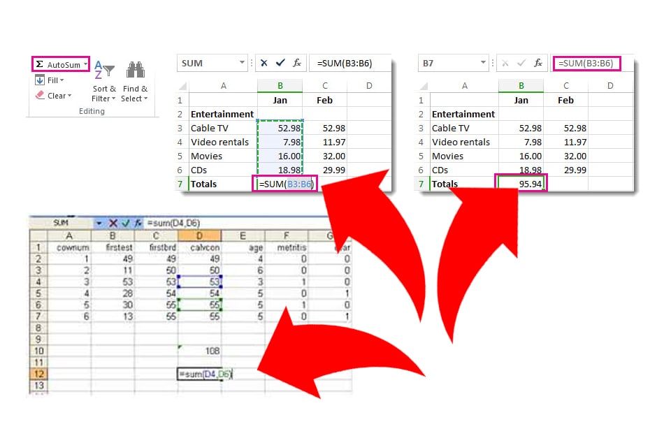
How to Add Cells in Excel to Sum Up Totals Automatically

Excel’s great for displaying data and even better at crunching numbers. Here’s how to add cells in Excel to sum up totals automatically… Even when you change the numbers.

A great feature that Excel has to offer is its use of formulas. Since Excel is often used to organize numerical data for a variety of operations, it can be beneficial to have an ‘addition’ function. In this guide, we are going to discuss the various ways we can add cells in Excel.

Why is the Addition Function Useful When You Need to Add Cells in Excel?

As we already know, in Excel Worksheets we can add columns. However, sometimes it is necessary to add cells that are not in columns or are not even next to each other.

For example, let’s say you are performing a survey to present data. You are interviewing random students to find out the most popular subjects taken in school. Your poll is anonymous, allows students to select only one option, and is organized by gender and grade levels Freshman, Sophomore, Junior, and Senior. The survey offers several subjects.

This survey is set up to give you a wide range of information and a variety of totals for you to examine. You could add these totals yourself, or you could use the many ways to add these numbers to Excel.

How to Add Cells in Excel: Method 1 (via Individual Table Cells)

In addition to adding columns in Excel, you can also add horizontally in rows. Let’s say you want to know how many senior males were surveyed. You can do this by adding up all the numbers in the Senior Male row. Let’s say the Senior Males row is row two in columns B2 through H2. One way to add your numbers is to select cell I2 and type the equals (=) sign, followed by the numbers in each cell in that row. For example, it may look something like this:

=5+6+2+7+0+9+1

Then, hit the enter button and you will get your total. While this method works, you will not be able to change the numbers in your cells without also changing your formula.

Because of this problem, it is better to enter the cells than the information within them. Rather than the above example, your formula will look similar to this:

=B2+C2+D2+E2+F2+G2+H2

When you hit Enter after typing this, you will still get your total. However, this time, you will be able to change the information in these cells, and the change will automatically affect the total.

How to Add Cells in Excel: Method 2 (Sum Function)

There is another method to adding rows. In this method, select your total cell. In our case, it has been cell I2. Type the equal (=) sign. Next, click the first cell in your row, or B2. This cell will become highlighted and appear next to the equal (=) sign. Then, type the plus (+) sign and click the next cells in the row. Continue this until you have clicked every cell in the row. Hit Enter to view your total.

Finally, rows can be added in the same SUM Function that we learned with columns. In your total cell, type =SUM. Then, type or click your beginning cell. Type the colon (:) mark and then type or click on the last cell in your row. It will look something like this:

=SUM(B2:H2)

Hit Enter when you have completed this function, and your total will show up. In this function, you can also change the values in each cell, and the changes will be reflected in the sum.

How to Add Cells in Excel: Method 3 (Adding Up Individual Cells In Different Rows and Columns)

The great thing about the addition function in Excel is that you not only get to add rows or columns. You can also add whatever cells you want to. Let’s stay with our survey example. Perhaps you want to examine precisely how many girls prefer math and science. Excel allows you to do this.

Label your first cell to maintain organization in your document. Click the cell next to it to begin your equation. Type the equal (=) sign, followed by all the cells you would like to add together. For example, your equation may look like this:

=C3+C5+C7+C9+D3+D5+D7+D9

Hit the Enter button when you are finished to get your total.

Of course, as we have already learned, it can be a bit tedious and take a while to type all of that. The alternate method would be to click instead of type. In your total cell, type the equal (=) sign. Then, click your first cell. Type the plus (+) sign and click your next cell. Continue this process until you have clicked all the cells you want to add. When you have selected all your cells, hit Enter to get your total.

Using this method allows you to select any cell that contains a numerical value. The values do not have to be in the same row or column or be next to each other. This method also allows you to change information in cells used in your formula. The modified data will automatically update the total to reflect the new numbers.

Conclusion

It was certainly good news to hear that we can add columns of information within our Excel Worksheets. It made life a lot easier and minimized the work we had to do.

Now, we see that we can also add rows as well as individual cells. This guide has expanded what we can do with the addition function. This function could be vital information when it comes to surveys, projects, and organizing business or personal information.

Follow this step by step guide to add cells in Excel using the addition function to its fullest, incorporating rows and cells into your skill set.

Excel without a Mac

I sold my 15″ MacBook Pro yesterday and am waiting on a 21.5″ iMac to arrive in 2-3 weeks. So no more adventures with Excel 2011 for a bit.

Time to dust off the Dell desktop and reacquaint myself with the “real” Excel. That of the Windows variety. I’m putting Excel 2003 in my rear view mirror (finally) and will focus on Excel 2007 and 2010.

I would love to get Excel 2013 and test it out, but the Dell will need to be replaced this year so I’ll wait until I have a new PC. I would like it to be a PC / Tablet combo machine with Windows 8, but am going to wait until the dust settles on the new operating system.

When upgrading to a new version of Windows I usually make it a practice to wait until after “service pack 1” is released before making the switch.

So Excel without a Mac is a survivable condition when you have a Windows PC for a backup. The converse is not true. Having a Mac without Excel would be the worst form of torture. Living with Numbers is not, in my opinion, a survivable condition. Excel on a Mac is a challenge, but nirvana when compared to Numbers.

Which leads me to wonder when the next version of Excel for the Mac will come out. I have high expectations: Power Pivot, Name Manager, Evaluate Formula dialog box, Status Bar Functions that aren’t circa Excel 2003, and elimination of the Menu bar.

However, my expectations might just be the result of some wishful thinking rooted in a dream state.

20130208-185246.jpg

Horizontal Dynamic Dependent Drop Down List Example

A Dynamic Dependent Drop Down List with a Horizontal Table Reference

I received a comment asking if a dynamic dependent drop-down list in Excel could have a list where the “table headers were actually rows and not columns?” Since I’ve already detailed how this is done in the article mentioned above, I’ll keep this short. The screen shot below is what I’ll be referencing. At the end of the post I’ll give a link to the file I used.

Conditional Drop Down List (Excel)

Horizontal Dynamic Dependent Drop Down List Example

There are two named ranges,

    1. 1)

myCategoryH

    1. that refers to the range E1:E3 and


    1. 2)

myTableH

    that refers to range F1:G3.

A defined name, myItemListH, is created with the following formula =INDEX(myTableH,MATCH(Sheet1!A2,myCategoryH,0),0) that will return a row that is matched by the contents of cell A2.

In cell A2, add a Data Validation list with the source being =myCategoryH. In cell B2, add a Data Validation list with the source being =myItemListH in the conditional drop down list from Excel.

Now you’re done.

Cell A2 will give you a drop-down list of Fruit, Vegetables, or Other Stuff. And cell B2 will read the value in cell A2, match and return the proper row number, and return an array of values for that row.

Two Ways to Use the INDEX Function to Return an Array

This is a simple case of using the INDEX function in a slightly different way. Normally, to return column 2 of a named range, you would use the following formula =INDEX(myTable,0,2). The zero means: return all rows (of column 2).

If you want to return row 2 of the named range you would use =INDEX(myTable,2,0). Here the zero means: return all columns (of row 2).

This comes from the Help section of the INDEX function where in Excel 2011 it reads:

If you set row_num or column_num to 0 (zero), INDEX returns the array of values for the entire column or row, respectively. To use values returned as an array, enter the INDEX function as an array formula in a horizontal range of cells for a row, and in a vertical range of cells for a column. To enter an array formula, press ⌘+RETURN.

Practical Considerations

Adding to each category list across columns is problematic. For one thing adding more data to the table will require inserting a column within the table range to avoid renaming the range. Obviously a standard Excel “Table” won’t work with this type of list. And if you have a very large spreadsheet the number of columns will become limiting long before the number of rows would.

Download the File

Horizontal-Dynamic-Dependent-Drop-Down-List.xlsx

How to Update a List or Range without OFFSET

I avoid the use of Volatile Functions, especially OFFSET, which is commonly used to update a list or range. They can slow down the operation of your workbook. For very large workbooks with lots of data, it can be significant and irksome.

Worksheet cells that use Data Validation for a drop-down list can simplify the input process, or be used to limit the available choices. But the list needs be expandable. Here are two primary ways to keep your data validation list automatically updated, without having to resort to using the OFFSET function.

Update Your List Range with VBA

Put your data validation drop-down cell on one worksheet and the reference list range on another worksheet. Example: Sheet1 contains a cell with data validation. Sheet2 contains a data range (the list) that is given a defined name of myList. Add some VBA code in the Sheet2 Deactivate routine to update the named range.


Private Sub Worksheet_Deactivate()
Dim rng As Range
Set rng = Sheet2.Range("myList").CurrentRegion
Set rng = rng.Offset(1, 0).Resize(rng.Rows.Count - 1, rng.Columns.Count)
rng.Name = "myList"
End Sub

This is an event-based programming technique, which I commonly use with Excel 2003.

Data Validation List Lookup 1 Sheet

Use Some Table INDEX Magic

This is a variation of the same thing, but no VBA programming is warranted. Instead, use a Table for your reference list data. Then create a defined name with the INDEX Function, and use that name for the data validation list.

Tables automatically update their ranges when expanded and the INDEX function will too. Example: Create the defined name myListFormula and use =INDEX(Table1,0,1) as the formula. Then when setting the data validation list, use =myListFormula as the list reference.

Data Validation List Lookup 2 Sheet

Example Worksheet

I’ve put together a workbook with the two examples listed above. The first technique, with VBA, uses two worksheets: Lookup 1 and Data 1. The Data 1 worksheet has the VBA code, which updates the named range when deactivated. You can add or subtract to this list and the data validation list on the Lookup 1 sheet will automatically be updated.

Both Lookup sheets have data validation in cell A2, which is a list of names. I’ve added another column for the city that uses a formula to get the right value from the list.

Lookup 1 Sheet

Lookup 1 Sheet

Data 2 with VBA Code

Data 2 Sheet with VBA Code

The second example uses Lookup 2 and Data 2 worksheets. The Table is on the Data 2 worksheet. When you add or subtract data from this Table and the defined name myListFormula will automatically update the data validation list on the Lookup 2 worksheet. Be sure to look at the Define Name dialog box (on the Mac) or the Name Manager (Windows) to see the INDEX formula.

Define Name Dialog Box

Download the file: Data_Validation_List_Update.xlsm

Since there is no OFFSET function, updating at random intervals, in either of these examples, I can rest easy. That’s one less thing to slow down your worksheet.

Analysis ToolPak AddIn

Check the Analysis ToolPak Add-In in Excel 2003 [VBA Code]

Analysis ToolPak AddInI recently began using the NETWORKDAYS function in Excel 2007, yet my file was going to be widely used by people with Excel 2003 (both are Windows versions). The NETWORKDAYS function is a standard function in Excel 2007, but with 2003 you have to install the Analysis ToolPak, otherwise you get an error.

The only way for me to avert an error with users who don’t have the Analysis TookPak installed in Excel 2003 is to use some VBA code that runs when the file is opened. I want to see if they are using a version of Excel older than 2007, check if they have the Analysis ToolPak installed, and then tell them, with a pop-up message, to install the Analysis ToolPak, so all the formulas will work correctly.

Create a Routine to Check for the Analysis ToolPak

Open the Visual Basic Editor (Alt+F11) then choose Insert > Module and enter the following VBA code.


Sub CheckToolPak()
''''''''''''''''''''''''''''''''''''''''''''''''''''''''''''''''''
' Checks to see if the Excel version comes before Excel 2007,
' if so then checks to see if the Analysis ToolPak is installed.
' If not, then notify the user and end the program.
'
' This is required because of the NETWORKDAYS formula
' that is used in the charts.
''''''''''''''''''''''''''''''''''''''''''''''''''''''''''''''''''
If CInt(Application.Version) < 12 Then If AddIns("Analysis ToolPak").Installed <> True Then
MsgBox "Please install the Analysis ToolPak." & vbCr & vbCr & _
"Choose Tools > Add-Ins... " & vbCr & _
"then check the box for Analyiss ToolPak, and click OK."
End
End If
End If
End Sub

The code is somewhat self-explainatory except that Application.Version returns a text value, hence you see the CInt function that converts that text value to an integer so that we can tell if the Excel version is less than 12, which is the version number of Excel 2007.

Create a Workbook Open Event

This will do the trick, but needs a trigger to call the routine. So double-click ThisWorkbook in the Project Explorer of the VBA Editor, then select the drop-down at the top-left of the window – where you see (General) – and select Workbook. The Private Sub Workbook_Open() subroutine will appear with no code.

Type in Call CheckToolPak and then save the file.


Private Sub Workbook_Open()
Call CheckToolPak
End Sub

Now when you open the file with Excel 2003, and don’t happen to have the Analysis TookPak installed, you get the following message.

Analysis ToolPak PopUp

If users have the Analysis ToolPak Add-In installed in Excel 2003 there is no message, nor if the user is using Excel 2007, 2010 or 2011.

Excel 2010 icon

An Excel Crossroads – Mac and Windows

Excel 2010 iconI bought a MacBook Pro and installed Windows 7 with Boot Camp Assistant so I could access the “normal” Excel. This was important to me at the time because I was doing Excel development work in versions 2003, 2007 and 2010 on a Windows PC.

MacBook ProI love my MacBook Pro, which I consider my computer of the future. It’s great for dealing with Photos, Movies, Music, and all of my iOS devices.

I purchased the Mac versions of Excel (2008 and 2011) but they seem like a mixture of the three Excel versions mentioned above, and can be very frustrating at times. There are a few things missing in the latest Excel Mac version, like the Name Manager and the Evaluate Formula dialog box, to name just two.

Despite these shortcomings, I’m seriously thinking about selling my desktop PC and going exclusively with the Mac. That’s the crossroads I’m at right now. Letting go of the PC, but keeping the Windows versions of Excel.

My Hangups

BootCamp allows me to run Windows, and the Excel versions I need, but is very restrictive in the sense that I have to shut down my Mac, then restart with BootCamp to run Windows 7. This is a real pain in the you-know-what.

There are other problems with running Windows on a Mac. For instance, I haven’t been able to get my Apple Magic Mouse to work with Windows 7. (Go figure.) And using Dropbox was the best way to get Excel files between Windows 7 and Mac OS X.

My Saving Grace

All of those issues were solved when I purchased the Parallels Desktop software for Mac. Now I can switch to Windows without having to shut down Mac OS X Lion. That’s just plain awesome!

I’m still getting used to how Parallels works, but this software is easily worth the purchase price. And my Apple Magic Mouse, just works.

Parallels Desktop on my MacBook Pro

Here’s a screen shot of the Parallels Desktop open on my MacBook Pro. You can see that I have Microsoft 2010 (Windows) open, but I want you to notice that I also have the Finder dialog box open.

Parallels Desktop

I dragged the Card Size Lookup.xlsx file from Finder onto the Excel 2010 (Windows) program and it opened. I then made a change to the spreadsheet and saved it. The file was saved back on my Mac from whence it came. This is the miracle of modern technology.

I still have lots of testing to do but it looks like the Parallels Desktop has made my life much, much easier. I know now which way to turn at the crossroads.

A Dynamic Dependent Drop Down List

A Dynamic Dependent Drop Down List in Excel

A Dynamic Dependent Drop Down ListThe other day I was reading a post over at the Contextures blog about Dynamic Dependent Excel Drop Downs and realized that using an Excel Table would provide an alternative method that is both simple and flexible. Tables are available in Excel versions 2007, 2010, and 2011.

In this post I’ll create a Table to hold the Category’s and Items, create three defined names using dynamic formulas, then use Data Validation to create two drop-down lists, the second being dependent upon the first.

Create at Reference Table

Here’s a Table with Category names in the header row and Items in the columns. I just typed in the information then converted to a Table.

Category and Item Table

Create a Dynamic Defined Name for Category List

Create a defined name for the Table1 Header row range by using the formula =Table1[#Headers]. Please note that Table1 is the name of the Table created in the step above.

This defined name is dynamic, meaning it will expand when more columns are added and shrink if any columns are deleted. It will return the header row of the Table, which we’ll use in the next step. I used myCategory for this defined name.

Create Category Defined Name

To create a defined name in Windows choose Formulas > Name Manager then click New…. On a Mac choose Insert > Name > Define…. This will bring up the New Name dialog box that looks like the Edit Name screen-shot shown above.

Create a Category Drop Down List with Data Validation

Type Category in cell A1 for the column heading. Next select cell A2, then choose Data > Data Validation > Data Validation… and in the Data Validation dialog box (shown below) select List from the Allow box, then type in =MyCategory in the Source box, and click OK.

My Category Data Validation

Now cell A2 has a drop down button that shows the Header row of the Table. (Don’t worry about extending this Data Validation down to more rows, we’ll take care of that later.)

Category Drop Down List

Column B will hold a drop-down list for the Item, which is dependent upon the Category. This takes two defined names to work properly.

Create the First Defined Name for Items

[Update: Select cell B2 before you follow this next step.]
Create a defined name with the following formula:

=INDEX(Table1,0,MATCH(Sheet1!A2,Table1[#Headers],0))

that I’ll name myItemList.

My Item List Defined Name

This formula will return a reference to the Table column that matches the Category selection in cell A2 on Sheet1.

If I use Data Validation to create a drop-down list with the myItemList defined name I’ll get eight items returned because Table1 has eight data rows. As you can see in the picture below, the Vegetables item list has two blank lines, and the Other Stuff item list has one blank line.  Not an elegant solution.

Table Column Full List

However, if you have a table that always has equal items (rows) in each column then this defined name formula will will work well for a Data Validation list.

Create a Second Defined Name for Items

We can create a second defined name that will give us a dynamic list with the exact count. The following OFFSET formula will do the trick.

=OFFSET(myItemList,0,0,COUNTA(myItemList),1)

This formula uses the first defined name (myItemList) but alters the height by counting the items. I named this defined name myItem, as you can see below in the Name Manager screen shot.

Name Manager for myList

Create an Item Drop Down List with Data Validation

Type Item in cell B1. Select cell B2 and open the Data Validation dialog box. Choose List and enter the following formula =myItem, then click OK.

Data Validation Item List

The result is a dynamic drop-down list in the Item column that’s dependent on the Category selection in column A, and returns the exact list.

Dynamic Dependent Drop Down List

Convert to a Table

Now it’s time to covert this to a Table, and by doing so the Data Validation will be preserved and automatically expand with the addition of more rows.

Select cell A2, then in Windows (Excel 2007, 2010) choose Insert > Table, verify the information in the Create Table dialog box, and click OK.

Create Table in Windows

On a Mac (Excel 2011), select cell A2 then choose Tables > New > Insert Table with Headers.

At this point I normally turn off the Data Filter because it’s rather annoying.

As your Table expands, with more rows or columns, this dynamic drop-down list will work just fine. To create a new row in the Table with Data Validation press the Tab key while the active cell is the last column of the last row.

Potential Problem with OFFSET

As you might have guessed the OFFSET formula depends on having items at the top of the list. Should your data have blank rows in the middle of the column, the drop-down won’t have all the items listed yet show blank cells in the list.

Blank Cells and Missing Data

In this case it’s best to use the first defined name (myItemList) in creating a dependent, drop-down list for Item. At least you’ll get all the data, even if it does have some blanks in the list.

Blank Cells and No Missing Data

Reference Table Location

For illustration purposes I’ve shown the reference Table on the same worksheet as the Category and Item Table. Normally I would place the reference Table on a different worksheet. In this instance none of the formulas would change.

[UPDATE]

I’ve had numerous questions about the details of this post so I’m putting a link here to download the file.

Excel 2010 Clipboard Group

Ribbon Home Tab Comparison – Excel 2010 Windows and 2011 Mac

I’ll review each hard-to-find item on the Ribbon’s Home Tab in Excel 2010 (Windows) and let you know where they are located in Excel 2011 (Mac). I’ve even got some nifty pictures to speed along that understanding.

Note: The Ribbons in Excel 2010 and 2007 (Windows) are interchangeable, but I’ll only refer to 2010 below.

Each Ribbon Tab in Excel is organized by Groups. In Excel 2010 the Groups are shown at the bottom of the Ribbon. In Excel 2011 the Groups appear at the top, which I prefer.

The Excel 2010 Home Tab

The Excel 2010 Home Tab has the following Groups: Clipboard, Font, Alignment, Number, Styles, Cells, and Editing.

Excel 2010 Home Tab Split

The Excel 2011 Home Tab

The Excel 2011 Home Tab has the following Groups: Edit, Font, Alignment, Number, Format, Cells, Themes.

Excel 2011 Home Tab Split

Similar Items on Both Home Tabs

The Font and Number Groups have the same items so there’s no need to review them. The Alignment and Cells Groups have the same items, and although there is some variation in the underlying drop-down options I won’t cover them in this post.

Items You Have to Hunt For in Excel 2011

I’ll review each item on the Excel 2010 Clipboard and Editing Groups, which have items located on the Edit Group and elsewhere in Excel 2011, and finish up with the Styles Group that relates to the Format Group.

Note: The Themes Group in Excel 2011 doesn’t exist on the Home Tab in Excel 2010, but can be found on the Page Layout Tab.

The Clipboard Group

From left to right, the Paste icon is the first thing you see on the Excel 2010 Home tab. It resides in the Clipboard Group. Luckily the Paste icon is located in the same position on the Excel 2011 Home tab, but in the Edit Group.

The other items in the Clipboard group — Cut, Copy, Format Painter — don’t have a counterpart in the Excel 2011 Ribbon, but rather you can find them on the Standard Toolbar.

Excel 2010 Clipboard Group

The Editing Group

The Editing Group items are a mixed bag that can be hard to find in Excel 2011 unless you add some toolbar icons to the Standard Toolbar.

Excel 2010 Editing Group

The Fill and Clear icons can be found in the Edit Group. AutoSum is located on the Formulas Tab in the Function Group. Sort & Filter exists as two separate icons in Excel 2011 and are located on the Data Tab in the Sort & Filter Group with an icon for Sort and one for Filter. The Find & Select icon is not on the Excel 2011 Ribbon but located on the right side above the toolbar in a different format: the Search in Sheet box, which has a drop-down button that will bring up options for Advanced Search and Replace.

Excel 2010 Search Box Menu

In Excel 2011 you can find Sort and Filter on the Data menu, and Find can be found on the Edit menu but all of these are less than optimal because they take you away from the Home tab and require more clicks on the mouse or taps on the trackpad than are necessary.

As you can see in the Editing Group picture above, I’ve added AutoSum, Sort, and Filter icons to the Standard Toolbar to make these functions only one click away. This is a lot easier than hunting them each time.

The Styles Group

In Excel 2010 the Styles Group mostly corresponds to the Format Group in Excel 2011.

Excel 2010 Styles Group

The Format As Table icon in Excel 2010 is located on the Tables Tab in the Table Styles Group in Excel 2011.

Summary

The first time you use the Excel 2011 Ribbon Home Tab can be a trying experience if you’ve just come over from Excel 2010 or 2007. Hopefully this little summary with pictures is a help to those of you who, like me, get frustrated with Excel for making things so different between Windows and Mac.

The Mini Toolbar in Excel

The Mini Toolbar is nice to have when you need to do basic formatting and the Home tab is not displayed. Introduced in Excel 2007 and available in Excel 2010, the Mini Toolbar appears above the shortcut menu when you right-click a cell, range, chart, shape or other object.

Note: There is no Mini Toolbar in Mac versions of Excel (2011, 2008).

The contents of the Mini Toolbar are dependent on the object you right-click.

Right-Click a Range

I frequently Bold and Center format my table headings, but when the Home tab is not displayed it’s quicker to use the Mini Toolbar.

Mini Toolbar Range Option

Right-Click a Chart

The Mini Toolbar has a drop-down list so you can pick the chart element you need to format. Below I’m changing the Plot background color.

Mini Toolbar Chart Options

Right-Click a Shape

There’s a lot of stuff you can format on a Shape object from the Mini Toolbar. Below I change the shape background fill color, change the font color, change the font to different sizes, then bold and center the text.

Mini Toolbar Shape Option

Quickly Format Something with the Mini Toolbar

Start playing around with the Mini Toolbar and you’ll find that it’s a time-saver. Especially when the formatting you need – Home tab, Chart Tools tab, Drawing Tools tab – isn’t currently selected.

Related Posts Plugin for WordPress, Blogger...