Nested IF Functions in Excel

The simplest Nested IF Function is using one IF Function inside another. When you have more than a few choices, nesting more IF Functions can quickly get complicated and, quite frankly, there are better ways to make decisions with Excel. Having said that, I have a simple method to account for the different choices that can arise with nested IF Functions.

Two Conditions – Binary Outcome

Two Conditions Binary Outcome
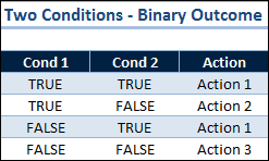
The IF Function evaluates a logical test to either TRUE or FALSE. A binary outcome. One condition requires only one IF Function.

With two conditions that both evaluate to TRUE/FALSE you must consider all possible outcomes.

This chart shows there are four different outcomes for Condition 1 and 2. I’ve added a third column to determine what action to take for each outcome.

One Nested IF Function

In this example three actions are required, which means one nested IF Function, so the Action column has the following formula:

=IF(Cond_2=TRUE,”Action 1″,IF(Cond_1=TRUE,”Action 2″,”Action 3″))

Which translates to: if condition 2 is TRUE then do action 1, or if condition 2 is  FALSE and condition 1 is TRUE then do action 2, or if condition 2 is FALSE and condition 1 is FALSE then do action 3.

How Many Actions are Required?

Having two conditions with binary outcomes doesn’t mean there will automatically be three actions for these four possible outcomes. The chart above is designed for you to determine how many actions are required, and then construct the IF statement logic.

Two Nested IF Functions

There could be four different actions needed, which would require two nested IF Functions. Assuming each of the four conditions above has a different outcome, and labeling each Action 1 through 4 from top to bottom, then the following formula will work:

=IF(Cond_1+Cond_2=2,”Action 1″,IF(Cond_1+Cond_2=0,”Action 4″,IF(Cond_1=TRUE,”Action 2″,”Action 3″)))

Which takes advantage of the fact that TRUE + TRUE = 2, FALSE + FALSE = 0, and either combination of TRUE + FALSE = 1.

Three Conditions – Binary Outcome

Three Conditions Binary Outcome
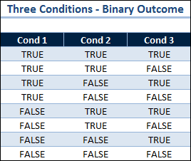
I rarely do more than two nested IF functions because they get complicated. Taking into account the binary nature each outcome, if there are N conditions, then there are 2N possible outcomes that must be accounted for with the formula logic.

I always put together a binary outcome chart when dealing with three conditions. Even if I don’t use nested IF Functions for a sloution, all the outcomes must be considered.

I simply add a column for what action needs to be taken and look to see where the commonality lies for a starting point, then try and compose something to fit.

Excel 2003 can nest up to 7 IF Functions, and Excel 2007 and 2010 both allow 64 nested IF Functions. How anybody could do that many Nested IF’s is beyond me.

If you’re trying to nest more IF Functions than I’ve shown here, I wish you Good Luck.

22 thoughts on “Nested IF Functions in Excel”

  1. Once you get into more than two conditions, it may pay to look at your desired outcomes and group them. Then treat each condition as a bit in a decision byte… Condition 1 = TRUE and Condition 2 = FALSE and Condition 3 = True => 101 base 2 or 5. Then use a SELECT CASE statement in a macro, or the CHOOSE statement in a cell, to come up with your desired outcome. So the cells formula would be something along the lines of =CHOOSE(EvaluatedConditions, Outcome1, Outcome2, Outcome3, etc).

    • I agree with you Eric. When I mentioned “better ways to make decisions” my first thought was to create a custom function using the SELECT CASE statement as you mentioned. And my second thought was the CHOOSE Function, although I don’t think I’ve ever used that one in a spreadsheet.

      As far as treating each condition as a bit in a decision byte, I get your meaning, but that’s slightly over my head. Thanks for the comment.

    • In this post I’m sticking with TRUE or FALSE outcomes for the IF Function to keep it simple. You can certainly use OR or AND Functions inside an IF Function, but then you run into an entirely different set of possible outcomes, which is a good topic for another article. Thanks for the comment.

  2. I’m a student at a university and we are working on excel and i am having a bit of difficulty we are given a 3×6 table example shown below and are required to “Create a formula/function as either … Failed, Passed, or achieved Honors. The cell should simply state: “Failed”, “Passed”, “Honors” – depending on their scores.”
    student test1 test2 test3
    Chelsea 60 65 80

    If any of the three scores falls below 60, the person fails the Law Exam. If the scores are all 80 or above, then the person is in the Honors ranking. If the scores are 60 or better but any one of the scores is below 80, they passed, but are not in the Honors ranking.

    how do i do this?

    • Assumes the Student “Chelsea” is in A2, and her grades for test1-3 are in B2:D2. For your “grade” cell (B5?), put in the following formula:

      =If(Min(B2:D2)=80,”Honors”,”Passed”))

      What this does is first check that any of her scores is less than 60. If it is, then she failed. Then, in the “FALSE” section of the first If statement, you check for the other two conditions. That second If statement checks to see if the minimum of her scores is greater than or equal to 80. If it is, then the other two scores are at least as good so she’s in the Honors section. And if she didn’t fail or isn’t in honors then she passed.

      Cheers,

      Eric

        • OK, it must be the greater than and equal sign…

          =If(Min(B2:D2)<60, "Failed",If(Min(B2:D2) GTE 80,"Honors","Passed"))

          Put a gt and an = sign in for GTE

          Eric

    • There are two conditions that require functions. Then put them into a Nested IF function and your done. Assume all the scores are in cells B2, C2, and D2. For the first condition, put a heading in cell E1 of Min<60. Then use the formula:

      =MIN(B2:D2)<60

      This will give a TRUE answer if all scores are above 79, which is the same thing as saying 80 or greater.

      Now for these two conditions you have only three outcomes, because if Min<60 is TRUE, then Honors? can't be TRUE, it's FALSE. The remaining two outcomes are if Min<60 is FALSE and Honors? is TRUE then they get Honors. And finally if Min<60 if FALSE and Honors? is FALSE they passed.

      Put the label Grade in cell G1 and in cell G2 the formula:

      =AND(B2>79,C2>79,D2>79)

      Putting everything together in one formula:

      =IF(MIN(B2:D2)<60,"Failed",IF(AND(B2>79,C2>79,D2>79),"Honors","Passed"))

      I hope that was clear.

  3. What about this formula ?

    =IF(AND(L3=D3,K3=”1-2″),E3,IF(AND(L3=D3,K3=”3-4″),F3,IF(AND(L3=D3,K3=5),G3,IF(AND(L3=D4,K3=”1-2″),E4,IF(AND(L3=D4,K3=”3-4″),F4,IF(AND(L3=D4,K3=5),G4,IF(AND(L3=D5,K3=”1-2″),E5,IF(AND(L3=D5,K3=”3-4″),f5,if(AND(L3=D5,K3=5),g5,if(AND(L3=D6,K3=”1-2″),e6,if(AND(L3=D6,K3=”3-4″),f6,if(AND(L3=D3,K3=5),g3,if(AND(L3=D3,K3=”1-2″),e3,if(AND(L3=D3,K3=”3-4″),f3,if(AND(L3=D3,K3=5),g3,if(AND(L3=D3,K3=”1-2″),e3,if(AND(L3=D3,K3=”3-4″),f3,if(AND(L3=D6,K3=5),g6,if(AND(L3=D7,K3=”1-2″),e7,if(AND(L3=D7,K3=”3-4″),f7,if(AND(L3=D7,K3=5),g7,if(AND(L3=D8,K3=”1-2″),e8,if(AND(L3=D8,K3=”3-4″),f8,if(AND(L3=D8,K3=5),g8,if(AND(L3=D9,K3=”1-2″),e9,if(AND(L3=D9,K3=”3-4″),f9,if(AND(L3=D9,K3=5),g9,if(AND(L3=D10,K3=”1-2″),e10,if(AND(L3=D10,K3=”3-4″),f10,if(AND(L3=D10,K3=5),g10,if(AND(L3=D11,K3=”1-2″),e11,if(AND(L3=D11,K3=”3-4″),f11,if(AND(L3=D11,K3=5),g11,if(AND(L3=D12,K3=”1-2″),e12,if(AND(L3=D12,K3=”3-4″),f12,if(AND(L3=D12,K3=5),g12,if(AND(L3=D13,K3=”1-2″),e13,if(AND(L3=D13,K3=”3-4″),f13,if(AND(L3=D13,K3=5),g13,if(AND(L3=D14,K3=”1-2″),e14,if(AND(L3=D14,K3=”3-4″),f14,if(AND(L3=D14,K3=5),g14,if(AND(L3=D15,K3=”1-2″),e15,if(AND(L3=D15,K3=”3-4″),f15,if(AND(L3=D15,K3=5),g15,if(AND(L3=D16,K3=”1-2″),e16,if(AND(L3=D16,K3=”3-4″),f16,if(AND(L3=D16,K3=5),g16,if(AND(L3=D17,K3=”1-2″),e17,if(AND(L3=D17,K3=”3-4″),f17,if(AND(L3=D17,K3=5),g17,if(AND(L3=D18,K3=”1-2″),e18,if(AND(L3=D18,K3=”3-4″),f18,if(AND(L3=D18,K3=5),g18,if(AND(L3=D19,K3=”1-2″),e19,if(AND(L3=D19,K3=”3-4″),f19,if(AND(L3=D19,K3=5),g19,if(AND(L3=D20,K3=”1-2″),e20,if(AND(L3=D20,K3=”3-4″),f20,if(AND(L3=D20,K3=5),g20,if(AND(L3=D21,K3=”1-2″),e21,if(AND(L3=D21,K3=”3-4″),f21,if(AND(L3=D21,K3=5),g21,if(AND(L3=D22,K3=”1-2″),e22,if(AND(L3=D22,K3=”3-4″),f22,if(AND(L3=D22,K3=5),g22,if(AND(L3=D23,K3=”1-2″),e23,if(AND(L3=D23,K3=”3-4″),f23,if(AND(L3=D23,K3=5),g23,if(AND(L3=D24,K3=”1-2″),e24,if(AND(L3=D24,K3=”3-4″),f24,if(AND(L3=D24,K3=5),g24,if(AND(L3=D25,K3=”1-2″),e25,if(AND(L3=D25,K3=”3-4″),f25,if(AND(L3=D25,K3=5),g25,if(AND(L3=D26,K3=”1-2″),e26,if(AND(L3=D26,K3=”3-4″),f26,if(AND(L3=D26,K3=5),g26,if(AND(L3=D27,K3=”1-2″),e27,if(AND(L3=D27,K3=”3-4″),f27,if(AND(L3=D27,K3=5),g27,if(AND(L3=D28,K3=”1-2″),e28,if(AND(L3=D28,K3=”3-4″),f28,if(AND(L3=D28,K3=5),g28,if(AND(L3=D29,K3=”1-2″),e29,if(AND(L3=D29,K3=”3-4″),f29,if(AND(L3=D29,K3=5),g29,if(AND(L3=D30,K3=”1-2″),e30,if(AND(L3=D30,K3=”3-4″),f30,if(AND(L3=D30,K3=5),g30,if(AND(L3=D31,K3=”1-2″),e31,if(AND(L3=D31,K3=”3-4″),f31,if(AND(L3=D31,K3=5),g31,if(AND(L3=D32,K3=”1-2″),e32,if(AND(L3=D32,K3=”3-4″),f32,if(AND(L3=D32,K3=5),g32,if(AND(L3=D33,K3=”1-2″),e33,if(AND(L3=D33,K3=”3-4″),f33,if(AND(L3=D33,K3=5),g33,if(AND(L3=D34,K3=”1-2″),e34,if(AND(L3=D34,K3=”3-4″),f34,if(AND(L3=D34,K3=5),g34,if(AND(L3=D35,K3=”1-2″),e35,if(AND(L3=D35,K3=”3-4″),f35,if(AND(L3=D35,K3=5),g35)

    How to make it simple and works ?

    It has more than 64 nest…

    thanks

    • I bow down to the brain-power that created this massive formula. If there’s more than three or four nested IF statements required, I resort to VBA code.

      • LOL… Come on… please help me out how to make an alternatives for this formula… Or maybe there is a way to modify the “64 nest” rule on the excel ?

        Thanks again

          • =IF(AND(L3=D3,K3=”1-2″),E3,IF(AND(L3=D3,K3=”3-4″),F3,IF(AND(L3=D3,K3=5),G3,IF(AND(L3=D4,K3=”1-2″),E4,IF(AND(L3=D4,K3=”3-4″),F4,IF(AND(L3=D4,K3=5),G4,IF(AND(L3=D5,K3=”1-2″),E5,IF(AND(L3=D5,K3=”3-4″),f5,if(AND(L3=D5,K3=5),g5,if(AND(L3=D6,K3=”1-2″),e6,if(AND(L3=D6,K3=”3-4″),f6,if(AND(L3=D3,K3=5),g3,if(AND(L3=D3,K3=”1-2″),e3,if(AND(L3=D3,K3=”3-4″),f3,if(AND(L3=D3,K3=5),g3,if(AND(L3=D3,K3=”1-2″),e3,if(AND(L3=D3,K3=”3-4″),f3,if(AND(L3=D6,K3=5),g6,if(AND(L3=D7,K3=”1-2″),e7,if(AND(L3=D7,K3=”3-4″),f7,if(AND(L3=D7,K3=5),g7,if(AND(L3=D8,K3=”1-2″),e8,if(AND(L3=D8,K3=”3-4″),f8,if(AND(L3=D8,K3=5),g8,if(AND(L3=D9,K3=”1-2″),e9,if(AND(L3=D9,K3=”3-4″),f9,if(AND(L3=D9,K3=5),g9,if(AND(L3=D10,K3=”1-2″),e10,if(AND(L3=D10,K3=”3-4″),f10,if(AND(L3=D10,K3=5),g10,if(AND(L3=D11,K3=”1-2″),e11,if(AND(L3=D11,K3=”3-4″),f11,if(AND(L3=D11,K3=5),g11,if(AND(L3=D12,K3=”1-2″),e12,if(AND(L3=D12,K3=”3-4″),f12,if(AND(L3=D12,K3=5),g12,if(AND(L3=D13,K3=”1-2″),e13,if(AND(L3=D13,K3=”3-4″),f13,if(AND(L3=D13,K3=5),g13,if(AND(L3=D14,K3=”1-2″),e14,if(AND(L3=D14,K3=”3-4″),f14,if(AND(L3=D14,K3=5),g14,if(AND(L3=D15,K3=”1-2″),e15,if(AND(L3=D15,K3=”3-4″),f15,if(AND(L3=D15,K3=5),g15,if(AND(L3=D16,K3=”1-2″),e16,if(AND(L3=D16,K3=”3-4″),f16,if(AND(L3=D16,K3=5),g16,if(AND(L3=D17,K3=”1-2″),e17,if(AND(L3=D17,K3=”3-4″),f17,if(AND(L3=D17,K3=5),g17,if(AND(L3=D18,K3=”1-2″),e18,if(AND(L3=D18,K3=”3-4″),f18,if(AND(L3=D18,K3=5),g18,if(AND(L3=D19,K3=”1-2″),e19,if(AND(L3=D19,K3=”3-4″),f19,if(AND(L3=D19,K3=5),g19,if(AND(L3=D20,K3=”1-2″),e20,if(AND(L3=D20,K3=”3-4″),f20,if(AND(L3=D20,K3=5),g20,if(AND(L3=D21,K3=”1-2″),e21,if(AND(L3=D21,K3=”3-4″),f21,if(AND(L3=D21,K3=5),g21,if(AND(L3=D22,K3=”1-2″),e22,if(AND(L3=D22,K3=”3-4″),f22,if(AND(L3=D22,K3=5),g22,if(AND(L3=D23,K3=”1-2″),e23,if(AND(L3=D23,K3=”3-4″),f23,if(AND(L3=D23,K3=5),g23,if(AND(L3=D24,K3=”1-2″),e24,if(AND(L3=D24,K3=”3-4″),f24,if(AND(L3=D24,K3=5),g24,if(AND(L3=D25,K3=”1-2″),e25,if(AND(L3=D25,K3=”3-4″),f25,if(AND(L3=D25,K3=5),g25,if(AND(L3=D26,K3=”1-2″),e26,if(AND(L3=D26,K3=”3-4″),f26,if(AND(L3=D26,K3=5),g26,if(AND(L3=D27,K3=”1-2″),e27,if(AND(L3=D27,K3=”3-4″),f27,if(AND(L3=D27,K3=5),g27,if(AND(L3=D28,K3=”1-2″),e28,if(AND(L3=D28,K3=”3-4″),f28,if(AND(L3=D28,K3=5),g28,if(AND(L3=D29,K3=”1-2″),e29,if(AND(L3=D29,K3=”3-4″),f29,if(AND(L3=D29,K3=5),g29,if(AND(L3=D30,K3=”1-2″),e30,if(AND(L3=D30,K3=”3-4″),f30,if(AND(L3=D30,K3=5),g30,if(AND(L3=D31,K3=”1-2″),e31,if(AND(L3=D31,K3=”3-4″),f31,if(AND(L3=D31,K3=5),g31,if(AND(L3=D32,K3=”1-2″),e32,if(AND(L3=D32,K3=”3-4″),f32,if(AND(L3=D32,K3=5),g32,if(AND(L3=D33,K3=”1-2″),e33,if(AND(L3=D33,K3=”3-4″),f33,if(AND(L3=D33,K3=5),g33,if(AND(L3=D34,K3=”1-2″),e34,if(AND(L3=D34,K3=”3-4″),f34,if(AND(L3=D34,K3=5),g34,if(AND(L3=D35,K3=”1-2″),e35,if(AND(L3=D35,K3=”3-4″),f35,if(AND(L3=D35,K3=5),g35))))))))))))))))))))))))))))))))))))

            thats the original formula….

          • I had to remove every instance of “1-2” and “3-4” because Excel wouldn’t accept the quotes, and then I got a warning that there were more than 64 levels of nesting. So I’m stuck.

  4. CCD : Your gigantic formula is nothing but finding the contents of a two way array. Where the values in L3 cell takes values from cell D3 to D35. And K3 cell takes fixed values 1-2, 3-4, & 5.
    Simply use MATCH function to find the row (Rx) and column (Cx) of the array your target value is in. Then use ” =CELL(“contents”,INDIRECT(ADDRESS(Rx, Cx)))

    Yes, it is that simple 🙂
    -Cheers

    • Your point is taken. However “simple” is a relative term. This post is written for people who struggle with more than one IF function. Given that premise, throwing in the MATCH, CELL, INDIRECT, and ADDRESS functions are difficult enough by themselves, yet together they are incomprehensible to my target audience.

  5. hello
    can u help me
    how i can write more than 22 conditions in excel as below was give me error

    =IF(Y3=$AN$4;”7/1″;IF(Y3=$AN$5;”7/1/1″;IF(Y3=$AN$6;”7/1/2″;IF(Y3=$AN$7;”7/1/3″;IF(Y3=$AN$8;”7/2″;IF(Y3=$AN$9;”7/3″;IF(Y3=$AN$10;”7/3/1″;IF(Y3=$AN$11;”7/3/2″;IF(Y3=$AN$12;”7/3/3″;IF(Y3=$AN$13;”7/4″;IF(Y3=$AN$14;”7/5″;IF(Y3=$AN$15;”7/6″;IF(Y3=$AN$16;”7/6/1″;IF(Y3=$AN$17;”7/6/2″;IF(Y3=$AN$18;”7/6/3″;IF(Y3=$AN$19;”7/7″;IF(Y3=$AN$20;”7/7/1″;IF(Y3=$AN$21;”7/7/2″;IF(Y3=$AN$22;”7/9″;IF(Y3=$AN$23;”7/9/1″;IF($AN$24;”7/9/2″;IF(Y3=$AN$25;”7/10″))))))))))))))))))))))

    • Instead of using a large number of IF statements, the VLOOKUP function would be much, much simpler if you can put your list in a table. The first column of the table holds the lookup data, “7/1” “7/1/1” etc. and the second column holds the answer you want to provide. I’ll send you an example worksheet with your data to show the details.

      Hope this helps.

Comments are closed.